Fitts D.D. - Principles of Quantum Mechanics[c] As Applied to Chemistry and Chemical Physics (1999)(en)

22 The wave function

of the particle is de®ned only as a range Äx and the momentum of the particle is de®ned only as a range Ä p. The product of these two ranges or `uncertainties' is of order " or larger. The exact value of the lower bound is dependent on how the uncertainties are de®ned. A precise de®nition of the uncertainties in position and momentum is given in Sections 2.3 and 3.10.

The Heisenberg uncertainty principle is a consequence of the stipulation that a quantum particle is a wave packet. The mathematical construction of a wave packet from plane waves of varying wave numbers dictates the relation (1.44). It is not the situation that while the position and the momentum of the particle are well-de®ned, they cannot be measured simultaneously to any desired degree of accuracy. The position and momentum are, in fact, not simultaneously precisely de®ned. The more precisely one is de®ned, the less precisely is the other, in accordance with equation (1.44). This situation is in contrast to classical-mechanical behavior, where both the position and the momentum can, in principle, be speci®ed simultaneously as precisely as one wishes.

In quantum mechanics, if the momentum of a particle is precisely speci®ed so that p p0 and Ä p 0, then the function A( p) is

		A( p) ä( p ÿ p0)
The wave packet (1.37) then becomes
	1	1		1
Ø(x, t) p2ð"		…ÿ1ä( p ÿ p0)ei( pxÿEt)=" d p p2ð" ei( p0 xÿEt)="			=
which is a plane	•••••••••		0=	•••••••••		".
	wave with wave number		p	" and angular frequency	E

Such a plane wave has an in®nite value for the uncertainty Äx. Likewise, if the position of a particle is precisely speci®ed, the uncertainty in its momentum is in®nite.

Another Heisenberg uncertainty relation exists for the energy E of a particle and the time t at which the particle has that value for the energy. The uncertainty Äù in the angular frequency of the wave packet is related to the uncertainty ÄE in the energy of the particle by Äù ÄE=", so that the

relation (1.25) when applied to a free particle becomes
ÄEÄt > "	(1:45)

Again, this relation arises from the representation of a particle by a wave packet and is a property of Fourier transforms.

The relation (1.45) may also be obtained from (1.44) as follows. The uncertainty ÄE is the spread of the kinetic energies in a wave packet. If Ä p is

small, then ÄE is related to Ä p by
	p2			p
ÄE Ä					Ä p	(1:46)
	2m			m

1.6 Young's double-slit experiment

23

The time Ät for a wave packet to pass a given point equals the uncertainty in

its position x divided by the group velocity vg
Äx				Äx			m
Ät								Äx	(1:47)
	vg			v			p

Combining equations (1.46) and (1.47), we see that ÄEÄt ÄxÄ p. Thus, the relation (1.45) follows from (1.44). The Heisenberg uncertainty relation (1.45) is treated more thoroughly in Section 3.10.

1.6 Young's double-slit experiment

The essential features of the particle±wave duality are clearly illustrated by Young's double-slit experiment. In order to explain all of the observations of this experiment, light must be regarded as having both wave-like and particlelike properties. Similar experiments on electrons indicate that they too possess both particle-like and wave-like characteristics. The consideration of the experimental results leads directly to a physical interpretation of SchroÈdinger's wave function, which is presented in Section 1.8.

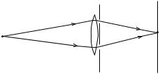
The experimental apparatus is illustrated schematically in Figure 1.8. Monochromatic light emitted from the point source S is focused by a lens L onto a detection or observation screen D. Between L and D is an opaque screen with two closely spaced slits A and B, each of which may be independently opened or closed.

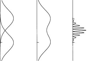
A monochromatic light beam from S passing through the opaque screen with slit A open and slit B closed gives a diffraction pattern on D with an intensity distribution IA as shown in Figure 1.9(a). In that ®gure the points A and B are directly in line with slits A and B, respectively. If slit A is closed and slit B open, the intensity distribution of the diffraction pattern is given by the curve labeled IB in Figure 1.9(a). For an experiment in which slit A is open and slit B is closed half of the time, while slit A is closed and slit B is open the other half of the time, the resulting intensity distribution is the sum of IA and IB, as shown in Figure 1.9(b). However, when both slits are open throughout an

D

L A

S

B

Figure 1.8 Diagram of Young's double-slit experiment.

24			The wave function
		IA			IA 1 IB
A			A			A

B IB B B

(a)

(b)

(c)

Figure 1.9 (a) Intensity distributions IA from slit A alone and IB from slit B alone. (b) The sum of the intensity distributions IA and IB. (c) The intensity interference pattern when slits A and B are open simultaneously.

experiment, an interference pattern as shown in Figure 1.9(c) is observed. The intensity pattern in this case is not the sum IA IB, but rather an alternating series of bright and dark interference fringes with a bright maximum midway between points A and B. The spacing of the fringes depends on the distance between the two slits.

The wave theory for light provides a satisfactory explanation for these observations. It was, indeed, this very experiment conducted by T. Young (1802) that, in the nineteenth century, led to the replacement of Newton's particle theory of light by a wave theory.

The wave interpretation of the interference pattern observed in Young's experiment is inconsistent with the particle or photon concept of light as required by Einstein's explanation of the photoelectric effect. If the monochromatic beam of light consists of a stream of individual photons, then each photon presumably must pass through either slit A or slit B. To test this assertion, detectors are placed directly behind slits A and B and both slits are opened. The light beam used is of such low intensity that only one photon at a time is emitted by S. In this situation each photon is recorded by either one detector or the other, never by both at once. Half of the photons are observed to pass through slit A, half through slit B in random order. This result is consistent with particle behavior.

How then is a photon passing through only one slit in¯uenced by the other slit to produce an interference pattern? A possible explanation is that somehow photons passing through slit A interact with other photons passing through slit

1.6 Young's double-slit experiment

25

B and vice versa. To answer this question, Young's experiment is repeated with both slits open and with only one photon at a time emitted by S. The elapsed time between each emission is long enough to rule out any interactions among the photons. While it might be expected that, under these circumstances, the pattern in Figure 1.9(b) would be obtained, in fact the interference fringes of Figure 1.9(c) are observed. Thus, the same result is obtained regardless of the intensity of the light beam, even in the limit of diminishing intensity.

If the detection screen D is constructed so that the locations of individual photon impacts can be observed (with an array of scintillation counters, for example), then two features become apparent. The ®rst is that only whole photons are detected; each photon strikes the screen D at only one location. The second is that the interference pattern is slowly built up as the cumulative effect of very many individual photon impacts. The behavior of any particular photon is unpredictable; it strikes the screen at a random location. The density of the impacts at each point on the screen D gives the interference fringes. Looking at it the other way around, the interference pattern is the probability distribution of the location of the photon impacts.

If only slit A is open half of the time and only slit B the other half of the time, then the interference fringes are not observed and the diffraction pattern of Figure 1.9(b) is obtained. The photons passing through slit A one at a time form in a statistical manner the pattern labeled IA in Figure 1.9(a), while those passing through slit B yield the pattern IB. If both slits A and B are left open, but a detector is placed at slit A so that we know for certain whether each given photon passes through slit A or through slit B, then the interference pattern is again not observed; only the pattern of Figure 1.9(b) is obtained. The act of ascertaining through which slit the photon passes has the same effect as closing the other slit.

The several variations on Young's experiment cannot be explained exclusively by a wave concept of light nor by a particle concept. Both wave and particle behavior are needed for a complete description. When the photon is allowed to pass undetected through the slits, it displays wave behavior and an interference pattern is observed. Typical of particle behavior, each photon strikes the detection screen D at a speci®c location. However, the location is different for each photon and the resulting pattern for many photons is in accord with a probability distribution. When the photon is observed or constrained to pass through a speci®c slit, whether the other slit is open or closed, the behavior is more like that of a particle and the interference fringes are not observed. It should be noted, however, that the curve IA in Figure 1.9(a) is the diffraction pattern for a wave passing through a slit of width comparable to the wavelength of the wave. Thus, even with only one slit open

26	The wave function

and with the photons passing through the slit one at a time, wave behavior is observed.

Analogous experiments using electrons instead of photons have been carried out with the same results. Electrons passing through a system with double slits produce an interference pattern. If a detector determines through which slit each electron passes, then the interference pattern is not observed. As with the photon, the electron exhibits both wave-like and particle-like behavior and its location on a detection screen is randomly determined by a probability distribution.

1.7 Stern±Gerlach experiment

Another experiment that relates to the physical interpretation of the wave function was performed by O. Stern and W. Gerlach (1922). Their experiment is a dramatic illustration of a quantum-mechanical effect which is in direct con¯ict with the concepts of classical theory. It was the ®rst experiment of a non-optical nature to show quantum behavior directly.

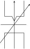
In the Stern±Gerlach experiment, a beam of silver atoms is produced by evaporating silver in a high-temperature oven and allowing the atoms to escape through a small hole. The beam is further collimated by passage through a series of slits. As shown in Figure 1.10, the beam of silver atoms then passes through a highly inhomogeneous magnetic ®eld and condenses on a detection plate. The cross-section of the magnet is shown in Figure 1.11. One pole has a very sharp edge in order to produce a large gradient in the magnetic ®eld. The atomic beam is directed along this edge (the z-axis) so that the silver atoms experience a gradient in magnetic ®eld in the vertical or x-direction, but not in the horizontal or y-direction.

Silver atoms, being paramagnetic, have a magnetic moment M. In a magnetic ®eld B, the potential energy V of each atom is

V ÿM . B

Between the poles of the magnet, the magnetic ®eld B varies rapidly in the x-

x

z

Oven Collimating		y
slits	Magnet	Detection

plate

Figure 1.10 Diagram of the Stern±Gerlach experiment.

1.7 Stern±Gerlach experiment

27

x

z

y

Magnet

Figure 1.11 A cross-section of the magnet in Figure 1.10.

direction, resulting in a force Fx in the x-direction acting on each silver atom. This force is given by

Fx ÿ	@V	M cos è	@B
	@x		@x

where M and B are the magnitudes of the vectors M and B and è is the angle between the direction of the magnetic moment and the positive x-axis. Thus, the inhomogeneous magnetic ®eld de¯ects the path of a silver atom by an amount dependent on the orientation angle è of its magnetic moment. If the angle è is between 08 and 908, then the force is positive and the atom moves in the positive x-direction. For an angle è between 908 and 1808, the force is negative and the atom moves in the negative x-direction.

As the silver atoms escape from the oven, their magnetic moments are randomly oriented so that all possible values of the angle è occur. According to classical mechanics, we should expect the beam of silver atoms to form, on the detection plate, a continuous vertical line, corresponding to a gaussian distribution of impacts with a maximum intensity at the center (x 0). The outer limits of this line would correspond to the magnetic moment of a silver atom

parallel (è 08)	and antiparallel (è 1808)	to the magnetic	®eld gradient
(@B=@x). What	is actually observed on the	detection plate	are two spots,

located at each of the outer limits predicted by the classical theory. Thus, the beam of silver atoms splits into two distinct components, one corresponding to è 08, the other to è 1808. There are no trajectories corresponding to intermediate values of è. There is nothing unique or special about the vertical direction. If the magnet is rotated so that the magnetic ®eld gradient is along the y-axis, then again only two spots are observed on the detection plate, but are now located on the horizontal axis.

The Stern±Gerlach experiment shows that the magnetic moment of each

28	The wave function

silver atom is found only in one of two orientations, either parallel or antiparallel to the magnetic ®eld gradient, even though the magnetic moments of the atoms are randomly oriented when they emerge from the oven. Thus, the possible orientations of the atomic magnetic moment are quantized, i.e., only certain discrete values are observed. Since the direction of the quantization is determined by the direction of the magnetic ®eld gradient, the experimental process itself in¯uences the result of the measurement. This feature occurs in other experiments as well and is characteristic of quantum behavior.

If the beam of silver atoms is allowed to pass sequentially between the poles of two or three magnets, additional interesting phenomena are observed. We describe here three such related experimental arrangements. In the ®rst arrangement the collimated beam passes through a magnetic ®eld gradient pointing in the positive x-direction. One of the two exiting beams is blocked (say the one with antiparallel orientation), while the other (with parallel orientation) passes through a second magnetic ®eld gradient which is parallel to the ®rst. The atoms exiting the second magnet are deposited on a detection plate. In this case only one spot is observed, because the magnetic moments of the atoms entering the second magnetic ®eld are all oriented parallel to the gradient and remain parallel until they strike the detection plate.

The second arrangement is the same as the ®rst except that the gradient of the second magnetic ®eld is along the positive y-axis, i.e., it is perpendicular to the gradient of the ®rst magnetic ®eld. For this arrangement, two spots of silver atoms appear on the detection plate, one to the left and one to the right of the vertical x-axis. The beam leaving the ®rst magnet with all the atomic magnetic moments oriented in the positive x-direction is now split into two equal beams with the magnetic moments oriented parallel and antiparallel to the second magnetic ®eld gradient.

The third arrangement adds yet another vertical inhomogeneous magnetic ®eld to the setup of the second arrangement. In this new arrangement the collimated beam of silver atoms coming from the oven ®rst encounters a magnetic ®eld gradient in the positive x-direction, which splits the beam vertically into two parts. The lower beam is blocked and the upper beam passes through a magnetic ®eld gradient in the positive y-direction. This beam is split horizontally into two parts. The left beam is blocked and the right beam is now directed through a magnetic ®eld gradient parallel to the ®rst one, i.e., oriented in the positive x-direction. The resulting pattern on the detection plate might be expected to be a single spot, corresponding to the magnetic moments of all atoms being aligned in the positive x-direction. What is observed in this case, however, are two spots situated on a vertical axis and corresponding to atomic magnetic moments aligned in equal numbers in both the positive and negative

1.8 Physical interpretation of the wave function

29

x-directions. The passage of the atoms through the second magnet apparently realigned their magnetic moments parallel and antiparallel to the positive y- axis and thereby destroyed the previous information regarding their alignment by the ®rst magnet.

The original Stern±Gerlach experiment has also been carried out with the same results using sodium, potassium, copper, gold, thallium, and hydrogen atoms in place of silver atoms. Each of these atoms, including silver, has a single unpaired electron among the valence electrons surrounding its nucleus and core electrons. In hydrogen, of course, there is only one electron about the nucleus. The magnetic moment of such an atom is due to the intrinsic angular momentum, called spin, of this odd electron. The quantization of the magnetic moment by the inhomogeneous magnetic ®eld is then the quantization of this electron spin angular momentum. The spin of the electron and of other particles is discussed in Chapter 7.

Since the splitting of the atomic beam in the Stern±Gerlach experiment is due to the spin of an unpaired electron, one might wonder why a beam of electrons is not used directly rather than having the electrons attached to atoms. In order for a particle to pass between the poles of a magnet and be de¯ected by a distance proportional to the force acting on it, the trajectory of the particle must be essentially a classical path. As discussed in Section 1.4, such a particle is described by a wave packet and wave packets disperse with time±the lighter the particle, the faster the dispersion and the greater the uncertainty in the position of the particle. The application of Heisenberg's uncertainty principle to an electron beam shows that, because of the small mass of the electron, it is meaningless to assign a magnetic moment to a free electron. As a result, the pattern on the detection plate from an electron beam would be suf®ciently diffuse from interference effects that no conclusions could be drawn.2 However, when the electron is bound unpaired in an atom, then the atom, having a suf®ciently larger mass, has a magnetic moment and an essentially classical path through the Stern±Gerlach apparatus.

1.8 Physical interpretation of the wave function

Young's double-slit experiment and the Stern±Gerlach experiment, as described in the two previous sections, lead to a physical interpretation of the wave function associated with the motion of a particle. Basic to the concept of the wave function is the postulate that the wave function contains all the

2This point is discussed in more detail in N. F. Mott and H. S. W. Massey (1965) The Theory of Atomic Collisions, 3rd edition, p. 215±16, (Oxford University Press, Oxford).

30	The wave function

information that can be known about the particle that it represents. The wave function is a complete description of the quantum behavior of the particle. For this reason, the wave function is often also called the state of the system.

In the double-slit experiment, the patterns observed on the detection screen are slowly built up from many individual particle impacts, whether these particles are photons or electrons. The position of the impact of any single particle cannot be predicted; only the cumulative effect of many impacts is predetermined. Accordingly, a theoretical interpretation of the experiment must involve probability distributions rather than speci®c particle trajectories. The probability that a particle will strike the detection screen between some point x and a neighboring point x dx is P(x) dx and is proportional to the range dx. The larger the range dx, the greater the probability for a given particle to strike the detection screen in that range. The proportionality factor P(x) is called the probability density and is a function of the position x. For example, the probability density P(x) for the curve IA in Figure 1.9(a) has a maximum at the point A and decreases symmetrically on each side of A.

If the motion of a particle in the double-slit experiment is to be represented by a wave function, then that wave function must determine the probability density P(x). For mechanical waves in matter and for electromagnetic waves, the intensity of a wave is proportional to the square of its amplitude. By analogy, the probability density P(x) is postulated to be the square of the absolute value of the wave function Ø(x)

P(x) jØ(x)j2 Ø (x)Ø(x)

On the basis of this postulate, the interference pattern observed in the doubleslit experiment can be explained in terms of quantum particle behavior.

A particle, photon or electron, passing through slit A and striking the detection screen at point x has wave function ØA(x), while a similar particle passing through slit B has wave function ØB(x). Since a particle is observed to retain its identity and not divide into smaller units, its wave function Ø(x) is postulated to be the sum of the two possibilities

Ø(x) ØA(x) ØB(x)

(1:48)

When only slit A is open, the particle emitted by the source S passes through slit A, thereby causing the wave function Ø(x) in equation (1.48) to change or collapse suddenly to ØA(x). The probability density PA(x) that the particle strikes point x on the detection screen is, then

PA(x) jØA(x)j2

and the intensity distribution IA in Figure 1.9(a) is obtained. When only slit B

1.8 Physical interpretation of the wave function

31

is open, the particle passes through slit B and the wave function Ø(x) collapses to ØB(x). The probability density PB(x) is then given by

PB(x) jØB(x)j2

and curve IB in Figure 1.9(a) is observed. If slit A is open and slit B closed half of the time, and slit A is closed and slit B open the other half of the time, then the resulting probability density on the detection screen is just

PA(x) PB(x) jØA(x)j2 jØB(x)j2

giving the curve in Figure 1.9(b).

When both slits A and B are open at the same time, the interpretation

changes. In this case, the probability density PAB(x) is

PAB(x) jØA(x) ØB(x)j2

2

(x)ØB(x)

j

j

j

j

ØA(x) 2

ØB(x)

Ø

Ø (x)ØA(x)

A

B

PA(x) PB(x) I AB(x)

(1:49)

where

I AB(x)

ØA(x)ØB(x)

ØB (x)ØA(x)

The probability density PAB(x) has an interference term I AB(x) in addition to the terms PA(x) and PB(x). This interference term is real and is positive for some values of x, but negative for others. Thus, the term I AB(x) modi®es the sum PA(x) PB(x) to give an intensity distribution with interference fringes as shown in Figure 1.9(c).

For the experiment with both slits open and a detector placed at slit A, the interaction between the wave function and the detector must be taken into account. Any interaction between a particle and observing apparatus modi®es the wave function of the particle. In this case, the wave function has the form of a wave packet which, according to equation (1.37), oscillates with time as eÿiEt=". During the time period Ät that the particle and the detector are interacting, the energy of the interacting system is uncertain by an amount ÄE, which, according to the Heisenberg energy±time uncertainty principle, equation (1.45), is related to Ät by ÄE > "=Ät. Thus, there is an uncertainty in the phase Et=" of the wave function and ØA(x) is replaced by eijØA(x), where j is real. The value of j varies with each particle±detector interaction and is totally unpredictable. Therefore, the wave function Ø(x) for a particle in this

experiment is
Ø(x) eijØA(x) ØB(x)	(1:50)
and the resulting probability density Pj(x) is