Rogers Computational Chemistry Using the PC

ITERATIVE METHODS

3

Radiation Density

If we think in terms of the particulate nature of light (wave-particle duality), the number of particles of light or other electromagnetic radiation (photons) in a unit of frequency space constitutes a number density. The blackbody radiation curve in Fig. 1-1, a plot of radiation energy density r on the vertical axis as a function of frequency n on the horizontal axis, is essentially a plot of the number densities of light particles in small intervals of frequency space.

We are using the term space as defined by one or more coordinates that are not necessarily the x, y, z Cartesian coordinates of space as it is ordinarily defined. We shall refer to 1-space, 2-space, etc. where the number of dimensions of the space is the number of coordinates, possibly an n-space for a many dimensional space. The r and n axes are the coordinates of the density–frequency space, which is a 2-space.

Radiation energy density is a function of both frequency and temperature r(n,T) so that the single curve in Fig. 1-1 implies one and only one temperature. Because frequency n times wavelength l is the velocity of light c ¼ nl ¼ 2:998 108 m s 1 (a constant), an equivalent functional relationship exists between energy density and wavelength. The energy density function can be graphed in a different but equivalent form r(l,T). The intensity I of electromagnetic radiation within any narrow frequency (or wavelength) interval is directly proportional to the number density of photons. It is also directly proportional to the power output of a light sensor or photomultiplier; hence both I and r are measurable quantities. Whenever one plots some function of radiation intensity I vs. n or l, the resulting curve is called a spectrum.

–3 mJ Density,Energy

Frequency

Figure 1-1 The Blackbody Radiation Spectrum. The short curve on the left is a Rayleigh function of frequency.

4	COMPUTATIONAL CHEMISTRY USING THE PC

Wien’s Law

In the late nineteenth century, Wien analyzed experimental data on blackbody radiation and found that the maximum of the blackbody radiation spectrum lmax shifts with the temperature according to the equation

lmaxT ¼ 2:90 10 3 m K

ð1-1Þ

where l is in meters and T is the temperature in kelvins.

The Planck Radiation Law

As Lord Rayleigh pointed out, the classical expression for radiation

rðn; TÞdn ¼ 8pkBT=c3 n2dn

ð1-2Þ

where kB is Boltzmann’s constant and c is the speed of light, must fail to express the blackbody radiation spectrum because r ¼ const: n2 is a segment of a parabola open upward (the short curve to the left in Fig. 1-1) and does not have a relative maximum as required by the experimental data. In late 1900, Max Planck presented the equation

dn
rðn; TÞdn ¼ 8phn=c3 n2 ehn=kBT 1	ð1-3Þ

where the units of rðn; TÞ are joules per cubic meter, as appropriate to an energy in joules per unit volume and h ¼ 6:626 10 34 J s (joule seconds) is a new constant, now called Planck’s constant. This equation expressed in terms of wavelength l is

dl
rðl; TÞ dl ¼ 8phc=l5 ehc=lkBT 1	ð1-4Þ

By setting dr=dl ¼ 0, one can differentiate Eq. (1-4) and show that the equation

e x þ		x
			¼ 1		ð1-5Þ
		5
holds at the maximum of Fig. 1-1 where
x ¼	hc				ð1-6Þ
	lkBT

Exercise 1-1

Given that c ¼ nl, show that Eqs. (1-3) and 1-4) are equivalent.

Exercise 1-2

Obtain Eq. (1-5) from Eq. (1-4).

ITERATIVE METHODS

5

COMPUTER PROJECT 1-1 Wien’s Law

The first computer project is devoted to solving Eq. (1-5) for x iteratively. When x has been determined, the remaining constants can be substituted into

lT ¼	hc		ð1-7Þ
	kBx
where h is Planck’s constant, c is the velocity of light in a vacuum,			2:998

108 m s 1, and kB ¼ 1:381 10 23 J K 1 is the Boltzmann constant. The result is a test of agreement between Planck’s theoretical quantum law and Wien’s displacement law [Eq. 1-1], which comes from experimental data.

Procedure. One approach to the problem is to select a value for x that is obviously too small and to increment it iteratively until the equation is satisfied. This is the method of program WIEN, where the initial value of x is taken as 1 (clearly, e 1 þ 15 < 1 as you can show with a hand calculator).

Program

PRINT ‘‘Program QWIEN’’ x = 1

10 x = x þ.1

a = EXP(-x) þ (x / 5) IF (a 1) < 0 THEN 10 PRINT a, x

END

In Program QWIEN (written in QBASIC, Appendix A), x is initialized at 1 and incremented by 0.1 in line 3, which is given the statement number 10 for future reference. Be careful to differentiate between a statement number like 10 x ¼ x þ .1 and the product 10 times x which is 10*x. A number a is calculated for x ¼ 1:1 that is obviously too small so (a 1) is less than 0 and the IF statement in line 5 sends control back to the statement numbered 10, which increments x by 0.1 again. This continues until (a 1) 0, whereupon control exits from the loop and prints the result for a and x.

There are, of course, many variations that can be written in place of Program QWIEN. You are urged to try as many as you can. Some suggestions are as follows:

a.Vary the size of the increment in x in program statement 10. Tabulate the increment size, the computed result for x, and the calculated Wien constant. Comment on the relationship among the quantities tabulated.

b.Change Program QWIEN so that the second term on the right of the line below statement 10 is x instead of x=5. Solve for this new equation. Change the line below statement 10 so that the second term on the left is x=2. Repeat with x=3, x=4, etc. Tabulate the values of x and the values of the denominator. Is x a sensitive function of the denominator in the second term of Program WIEN?

6	COMPUTATIONAL CHEMISTRY USING THE PC

c.Devise and discuss a scheme for more efficient convergence. For example, some scheme that uses large increments for x when x is far away from convergence and small values for the increment in x when x is near its true value would be more efficient than the preceding schemes. How, in more detail, could this be done? Try coding and running your scheme.

d.Another coding scheme can be used in True BASIC (Appendix A)

Program

PRINT ‘‘Program TWIEN’’ let X ¼ 1

do

let X ¼ X þ .1

let A ¼ exp(-X) þ X / 5 loop until (A 1) > 0 PRINT A, X

END

The program contains a ‘‘do loop’’ that iterates the statements within the loop until the condition (A 1) < 0 is true. Try moving the ‘‘do’’ statement around in the program to see what changes in the output. Explain. If you encounter an ‘‘infinite loop,’’ True BASIC has a STOP statement to get you out.

It is good practice to translate programs in one BASIC (QBASIC or True BASIC) to programs in the other if you have both interpreters. Note that the statement X ¼ X þ .1 in both programs makes no sense algebraically, but in BASIC it means, ‘‘take the number in memory register X, add 0.1 to it and store the result back in register X.’’ If you are not familiar with coding in BASIC, an hour or so with an instruction manual should suffice for the simple programs used in the first half of this book. By all means, look at the programs on the Wiley website.

COMPUTER PROJECT 1-2 Roots of the Secular Determinant

Later in this book, we shall need to find the roots of the secular matrix

		42 9x		12 2x					ð		Þ
		210	42x	42	9x					1-8
One way of obtaining the roots is to expand the determinantal equation
		42	9x 12		2x			¼ 0	ð1-9Þ
	210		42x	42		9x

To do this, multiply the binomials at the top left and bottom right (the principal diagonal) and then, from this product, subtract the product of the remaining two elements, the off-diagonal elements ð42 9xÞ. The difference is set equal to zero:

ð210 42xÞð12 2xÞ ð42 9xÞ2 ¼ 0

ð1-10Þ

ITERATIVE METHODS

7

This equation is a quadratic and has two roots. For quantum mechanical reasons, we are interested only in the lower root. By inspection, x ¼ 0 leads to a large number on the left of Eq. (1-10). Letting x ¼ 1 leads to a smaller number on the left of Eq. (1-10), but it is still greater than zero. Evidently, increasing x approaches a solution of Eq. (1-10), that is, a value of x for which both sides are equal. By systematically increasing x beyond 1, we will approach one of the roots of the secular matrix. Negative values of x cause the left side of Eq. (1-10) to increase without limit; hence the root we are approaching must be the lower root.

Program

PRINT ‘‘Program QROOT’’ x ¼ 0

20 x ¼ x þ 1

a ¼ (210 - 42 * x) * (12 - 2 * x) - (42 - 9 * x)^2

IF a > 0 GOTO 20

PRINT x: END

Program QROOT increments x by 1 on each iteration. It prints out 5 when the polynomial on the right of line 4 is greater than 0. We have gone past the root because x is too large. The program did not exit from the loop on x ¼ 4, but it did on x ¼ 5, so x is between 4 and 5. By letting x ¼ 4 in the second line and changing the third line to increment x by 0.1, we get 5 again so x is between 4.9 and 5.0. Letting x ¼ 4:9 with an increment of 0.01 yields 4.94 and so on, until the increment 0.00001 yields the lower root x ¼ 4:93488.

Although we will not need it for our later quantum mechanical calculation, we may be curious to evaluate the second root and we shall certainly want to check to be sure that the root we have found is the smaller of the two. Write a program to evaluate the left side of Eq. (1-10) at integral values between 1 and 100 to make an approximate location of the second root. Write a second program to locate the second root of matrix Eq. (1-10) to a precision of six digits. Combine the programs to obtain both roots from one program run.

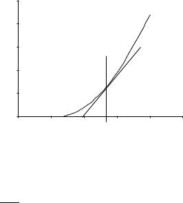
The Newton--Raphson Method

The root-finding method used up to this point was chosen to illustrate iterative solution, not as an efficient method of solving the problem at hand. Actually, a more efficient method of root finding has been known for centuries and can be traced back to Isaac Newton (1642–1727) (Fig. 1-2).

Suppose a function of x, f(x), has a first derivative f 0(x) at some arbitrary value of x, x0. The slope of f(x) is

	f 0	ð	x	Þ ¼	f ðx0Þ	ð	1-11	Þ
					ðx0 x1Þ

8	COMPUTATIONAL CHEMISTRY USING THE PC

f(x)

f(x0)

x1	x0	x

Figure 1-2 The First Step in the Newton–Raphson Method.

	whence
	x			x		f ðx0Þ	ð	1-12	Þ
		1	¼		0	f 0ðxÞ

The intersection of the slope and the x axis at x1 is closer to the root f(x) ¼ 0 than x0 was. By repeating this process, one can arrive at a point xn arbitrarily close to the root.

Exercise 1-3

Carry out the first two iterations of the Newton–Raphson solution of the polynomial Eq. (1-10).

Solution 1-3

The polynomial (1-10) can be written

x2 56x þ 252 ¼ 0

ð1-13Þ

The first derivative is

2x 56 ¼ 0

Starting at x0 ¼ 0

252
x1 ¼ x0				¼ 4:5
		56
and the second step yields
x2 ¼ 4:5		47				¼ 4:93085	ð1-14Þ
		20:25

ITERATIVE METHODS

9

This approximates the root x ¼ 4:93488 from Program QROOT in only two steps. Solution by the quadratic equation yields x ¼ 4:93487.

PROBLEMS

1.Show that Eq. (1-12) is the same as Eq. (1-11).

2.The energy of radiation at a given temperature is the integral of radiation density over all frequencies

ðn

E ¼ rðn; TÞdn

0

Find E from the known integral

ð0	ex 1 dx ¼	15
1	x3		p4

and compare the result with the Stefan–Boltzmann law

E ¼	4s		T	4
	c

where c is the velocity of light and s is an empirical constant equal to 5:67 10 8 J m 2 s 1. Just in case the value of the ‘‘known integral’’ is not obvious to you (it isn’t to me, either), we shall determine it numerically in another problem.

3.Analysis of the electromagnetic radiation spectrum emanating from the star Sirius shows that lmax ¼ 260 nm. Estimate the surface temperature of Sirius.

Numerical Integration

The term ‘‘quadrature’’ was used by early mathematicians to mean finding a square with an area equal to the area of some geometric figure other than a square. It is used in numerical integration to indicate the process of summing the areas of some number of simple geometric figures to approximate the area under some curve, that is, to approximate the integral of a function. We include numerical integration among the iterative methods because the integration program we shall use, following Simpson’s rule (Kreyszig, 1988), iteratively calculates small subareas under a curve f (x) and then sums the subareas to obtain the total area under the curve.

This discussion will be limited to functions of one variable that can be plotted in 2-space over the interval considered and that constitute the upper boundary of a well-defined area. The functions selected for illustration are simple and wellbehaved; they are smooth, single valued, and have no discontinuities. When discontinuities or singularities do occur (for example the cusp point of the 1s hydrogen orbital at the nucleus), we shall integrate up to the singularity but not include it.

10	COMPUTATIONAL CHEMISTRY USING THE PC

Contrary to the impression that one might have from a traditional course in introductory calculus, well-behaved functions that cannot be integrated in closed form are not rare mathematical curiosities. Examples are the Gaussian or standard error function and the related function that gives the distribution of molecular or atomic speeds in spherical polar coordinates. The famous blackbody radiation curve, which inspired Planck’s quantum hypothesis, is not integrable in closed form over an arbitrary interval.

Heretofore, the integral of a function of this kind was usually approximated by expressing it as an infinite series and evaluating some arbitrarily limited number of terms of the series. This always leads to a truncation error that depends on the number of terms retained in the sum before it is cut off (truncated). Numerical integration may be used instead of series solution when the analytical form of the function is known but not integrable or when the analytical form of the function is not known because the functional relationship exists as an instrument plot or a collection of paired measurements. This is the common case for data that have been obtained in an experimental setting. An example is the function describing a chromatographic peak, which may or may not approximate a Gaussian function.

We shall use the term analytical form to indicate a closed algebraic expression such as

y ¼ x2

ð1-15Þ

as contrasted to functions that are expressed as an infinite series, for example,

CP ¼ a þ bT þ cT2 þ dT3 þ

ð1-16Þ

Equation (1-15) is an analytical form that has a closed integral. The Gaussian function

f ðxÞ ¼ ð2pÞ 1=2 ez2=2

ð1-17Þ

is a closed analytical form but it has no closed integral. (Try to integrate it!) Several related ‘‘rules’’ or algorithms for numerical integration (rectangular rule,

trapezoidal rule, etc.) are described in applied mathematics books, but we shall rely on Simpson’s rule. This method can be shown to be superior to the simpler rules for well-behaved functions that occur commonly in chemistry, both functions for which the analytical form is not known and those that exist in analytical form but are not integrable.

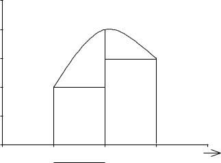
Simpson’s Rule

In applying Simpson’s rule, over the interval [a, b] of the independent variable, the interval is partitioned into an even number of subintervals and three consecutive points are used to determine the unique parabola that ‘‘covers’’ the area of the first

ITERATIVE METHODS

11

4

F(x)	1

3

2

xi

xi+1

xi+2

x

w

Figure 1-3 Areas Under a Parabolic Arc Covering Two Subintervals of a Simpson’s Rule Integration.

subinterval pair (see	Fig. 1-3). The area under this parabolic arc is	31wð f ðxiÞ þ
4f ðxiþ1Þ þ f ðxiþ2ÞÞ.	Summing for successive subinterval pairs over	the entire

interval constitutes the method known as Simpson’s rule. Looking at the formula below, one anticipates that an iterative loop will implement it on a microcomputer

ða f ðxÞdx ¼	31 wð f ðx0Þ þ 4f ðx1Þ þ 2f ðx2Þ þ 4f ðx3Þ þ
b
	þ 2f ðxn 2Þ þ 4f ðxn 1Þ þ f ðxnÞÞ	ð1-18Þ

Exercise 1-14

Show that the area under a parabolic arc that is convex upward is 13wð f ðxiÞ þ 4f ðxiþ1Þ þ f ðxiþ2ÞÞ, where w is the width of the subinterval xiþ1 xi.

Solution 1-4

The area under a parabolic arc concave upward is 13bh, where b is the base of the figure and h is its height. The area of a parabolic arc concave downward is 23bh. The areas of parts of the figure diagrammed for Simpson’s rule integration are shown in Fig. 1-3.

The area A under the parabolic arc in Fig. 1-3 is given by the sum of four terms:

A¼ 23 wð f ðxiþ1Þ f ðxiÞÞ þ wf ðxiÞ þ wð f ðxiþ2Þ þ 23 wð f ðxiþ1Þ f ðxiþ2ÞÞ

¼wð23 f ðxiþ1Þ þ 13 f ðxiÞ þ 23 f ðxiþ1Þ þ 13 f ðxiþ2ÞÞ

¼13 wð f ðxiÞ þ 4f ðxiþ1Þ þ f ðxiþ2ÞÞ

which was to be proven.

12	COMPUTATIONAL CHEMISTRY USING THE PC

Our Simpson’s rule program is written in QBASIC (Appendix A). Today’s computer world is full of complicated and expensive software, some of which we shall use in later chapters. Unfortunately, it is not hard to find software that is overpriced and overwritten (which we shall not use). Although it is not appropriate to recommend software in a book of this kind, the simple software used here has been used for several years in both a teaching and a research setting. It works.

More complicated and expensive programs are not necessarily better programs. One author recently described BASIC as a ‘‘primitive’’ language. Be that as it may, BASIC is ideal for solving simple problems. A hammer is a primitive tool. I wonder what our author friend would use to drive a nail.

Program QSIM is more general than any of the programs we have used to this point. By changing the define function statement DEF fna in line 8 of Program QSIM, one can obtain the integral of any well-behaved function between the limits a and b, which are specified in the interactive input to line 5. The term ‘‘interactive’’ is used here to denote interaction between the system and the operator (you). Line 6 is part of an INPUT statement requiring a response from you. The program will not run until you have specified the limits of integration, a and b along with n, the number of subintervals you wish to break the interval into. (The input numbers are separated by commas.) Note that statement 7 takes the subintervals in pairs so n must be an even number for the system to produce the correct integral. We are using the term ‘‘system’’ to denote both the hardware and software (hardware þ software ¼ system).

As an interesting beginning integration, let us determine the integral

ðb ð10

f ðxÞdx ¼ 100 x2 dx

a0

over the interval [0, 10] We can solve this integral by conventional means as a check on the result of numerical integration.

ð0	100 x2 dx ¼ 100x 3	0	¼ 1000	3 ¼ 666:667
10	x3	10		1000

Program

CLS

PRINT ‘‘Program QSIM’’

PRINT ‘‘Simpson’s Rule integration of the area under y ¼ f(x)’’ DEF fna (x) ¼ 100 - x ^ 2 0***DEF fna lets you put any function you like here.

PRINT ‘‘input limits a, and b, and the number of iterations desired n’’

INPUT a, b, n d ¼ (b - a) / n

FOR x ¼ a þ d TO b STEP 2 * d