Rogers Computational Chemistry Using the PC

ITERATIVE METHODS

13

sum ¼ sum þ 4 * fna(x) þ 2 * fna(x - d): NEXT x PRINT: PRINT: PRINT ‘‘RESULTS’’: PRINT

PRINT: PRINT ‘‘The interval is’’ ; a; ‘‘to’’; b; ‘‘’ ’ PRINT: PRINT ‘‘The number of iterations is ¼’’; n; ‘‘’’ a ¼ d / 3 * (fna(a) þ sum - fna(b))

PRINT: PRINT ‘‘Numerical integration yields’’, a: END

Names of programs written in QBASIC begin with Q. Programs written in True BASIC begin with T. Program QSIM differs from Programs QWIEN and QROOT in having more documentation. Documentation is used to make the program and the output easier for the operator to read. It is useful when a program is passed along to a colleague who was not in on the writing and may have difficulty understanding the logic of it. The CLS statement clears the screen, followed by a number of PRINT statements that should be obvious from context. Note that a full colon : is equivalent to a new line. Nothing enclosed in full quotes ‘‘ influences the functioning of the numerical part of the program. The prime or apostrophe ’ in line 4 instructs the system to ignore anything following it on the same line.

Efficiency and Machine Considerations

We selected a simple test function for integration. The function f ðxÞ ¼ 100 x2 is a smooth, monotonically decreasing parabolic curve over the interval [0, 10]. It has a closed definite integral over this interval of 666.667 units. The function is wellbehaved, and integration is easy over the first half of the interval but not so easy over the second half of the interval owing to its increasing steepness. (Note that steep functions can be integrated by an algorithm that sums horizontal slices of the area under the curve rather than vertical ones.)

The approximation to the closed integral improves as the number of iterations increases up to a point. The actual values in Table 1-1 may be system specific, that is, different hardware and software combinations may give slightly different results because of different ways of storing numbers. One is tempted to think of approximations as getting better without limit, the sum approaching the integral

Table 1-1 Approach of the Area Sum of Program QSIM to 666.667

Iterations (Subintervals)*
10	100	1000	10000	100000	1000000
Area sum**
733.73	673.33	667.33	666.75	666.84	665.82

* Large numbers may be input as exponentials, for example, 1e6 ¼ 1 106. ** May be system specific.

14	COMPUTATIONAL CHEMISTRY USING THE PC

as Achilles approached the tortoise. This does not occur, however, because of machine rounding error. (Only so many digits can be stored on a chip.) The last few entries in Table 1-1 show that for very many iterations, the area sum begins to diverge from, rather than approach, the integral it is supposed to represent (see also Norris, 1981). Keep rounding error in mind when writing programs with many iterations.

Elements of Single-Variable Statistics

When we report the result of a measurement x, there are two things a person reading the report wants to know: the magnitude (size) of the measurement and the reliability of the measurement (its ‘‘scatter’’). If measuring errors are random, as they very frequently are, the magnitude is best expressed as the arithmetic mean m of N repeated trials xi

	¼	P	ð		Þ
m		xi		1-19
		N
and the reliability is best expressed as the standard deviation
	¼	s	ð		Þ
		P
s		ðxi mÞ2		1-20

N

These equations apply when an entire population is available for measurement. The most common situation in practical problems is one in which the number of measurements is smaller than the entire population. A group of selected measurements smaller than the population is called a sample. Sample statistics are slightly different from population statistics but, for large samples, the equations of sample statistics approach those of population statistics.

If very many measurements are made of the same variable x, they will not all give the same result; indeed, if the measuring device is sufficiently sensitive, the surprising fact emerges that no two measurements are exactly the same. Many measurements of the same variable give a distribution of results xi clustered about their arithmetic mean m. In practical work, the assumption is almost always made that the distribution is random and that the distribution is Gaussian (see below).

Decision Making

A simple decision-making problem is: I measure variable x of a population A and the same variable x of a population B. I get (slightly) different results. Is there a real difference between populations A and B based on the difference in measurements, or am I only seeing different parts of the distributions of identical populations?

A similar decision-making problem consists of very many measurements of variable x on a large sample from population A, followed by a single measurement of the same property x of an individual. The single measurement will not be

ITERATIVE METHODS

15

precisely at the arithmetic mean of the large population. The question is whether the difference between m for the large population and measurement x indicates that the individual is not from the test population (is abnormal) or whether the deviation can be ascribed to a normal statistical fluctuation.

The second decision-making situation is very close to the problem presented in medical diagnosis in which we wish to know whether a patient is a member of the healthy general population or not. We shall apply Gaussian statistics to a diagnostic problem involving risk to a patient of atherosclerosis, given the blood cholesterol analysis of very many normal patients to which we compare the blood cholesterol analysis of the individual patient. In Computer Project 1-3, the patient is known to have a high blood cholesterol level but the problem is whether the measured level is sufficiently far from the mean of the normal population to be dangerous or whether it is only the random fluctuation we expect to see in some normal patients.

The Gaussian Distribution

The Gaussian distribution for the probability of random events is

!

p x		1	exp		ðxi mÞ2	ð	1-21	Þ
					2s2
ð Þ ¼ p

2ps

It is widely used in experimental chemistry, most commonly in statistical treatment of experimental uncertainty (Young, 1962). For convenience, it is common to make the substitution

z ¼ xi s m ð1-22Þ

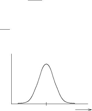
With this substitution, distributions having different m and s can be compared by using the same curve, frequently called the normal curve (Fig. 1-4).

(z)p

0z

Figure 1-4 The Gaussian Normal Distribution.

16	COMPUTATIONAL CHEMISTRY USING THE PC

ab

(z)p

0

z

Figure 1-5 An Interval [a, b] on the Gaussian Normal Distribution.

The integral of the Gaussian function over the interval [a, b] in a one-

dimensional probability space z is
pðzÞ ¼ p2p	ða e z =2dz	ð1-23Þ
1	b
	2

Equation (1-23) gives the probability of an event occurring within an arbitrary interval [a, b] (Fig. 1-5). Equation (1-23) has been ‘‘normalized’’ by choosing the right premultiplying constant p12p to make the integral over all space [ 1; 1] come out to 1.00 . . . . (see Problems) so the probability over any smaller interval [a, b] has a value not less than zero and not more than one.

The integral of the Gaussian distribution function does not exist in closed form over an arbitrary interval, but it is a simple matter to calculate the value of p(z) for any value of z, hence numerical integration is appropriate. Like the test function, f ðxÞ ¼ 100 x2, the accepted value (Young, 1962) of the definite integral (1-23) is approached rapidly by Simpson’s rule. We have obtained four-place accuracy or better at millisecond run time. For many applications in applied probability and statistics, four significant figures are more than can be supported by the data.

The iterative loop for approximating an area can be nested in an outer loop that prints the area under the Gaussian distribution curve for each of many increments in z. If the output is arranged in appropriate rows and columns, a table of areas under one half of the Gaussian curve can be generated, for example, from 0.0 to 3.0 z, resulting in printed values of the area at intervals of 0.01 z. This is suggested to the interested reader as an exercise. We generated a 400-entry table in a negligible run time. The Gaussian function is symmetrical, so knowing one half of the curve

ITERATIVE METHODS

17

means that we know the other half as well. The practical value of generating a table of Gaussian areas is small because many such tables are available in statistics books. The method, however, can be applied to derivative functions of the Gaussian function with only minor modifications, resulting in generation of tables of considerable practical importance (see below).

COMPUTER PROJECT 1-3 j Medical Statistics

The first application of the Gaussian distribution is in medical decision making or diagnosis. We wish to determine whether a patient is at risk because of the high cholesterol content of his blood. We need several pieces of input information: an expected or normal blood cholesterol, the standard deviation associated with the normal blood cholesterol count, and the blood cholesterol count of the patient. When we apply our analysis, we shall arrive at a diagnosis, either yes or no, the patient is at risk or is not at risk.

But decision making in the real world isn’t that simple. Statistical decisions are not absolute. No matter which choice we make, there is a probability of being wrong. The converse probability, that we are right, is called the confidence level. If the probability for error is expressed as a percentage, 100 (% probability for error) ¼ % confidence level.

The Problem. Suppose that the total serum cholesterol level in normal adults has been established as 200 mg/100 mL (mg%) with a standard deviation of 25 mg%, that is, m ¼ 200 and s ¼ 25. (Please distinguish between mg% and % probability.) A patient’s serum is analyzed for cholesterol and found to contain 265 mg% total cholesterol.

a.May we say at the 0.95 (95%) confidence level that the patient’s cholesterol is abnormally elevated, or is this just a chance fluctuation in a normal patient? To do this, we must first calculate z and then show that the patient’s cholesterol level is greater than or less than that of 95% of normal patients. For the reading to be abnormally elevated with 95% confidence, the z-value must be in an area above the 95% limit of the z-curve. The 95% limit of the z-curve is that point on the z-axis with 95% of normal cholesterol measurements below it and 5% of the measurements above it (Fig. 1-6).

b.May we reach the same conclusion at the 0.99% confidence level?

c.If the patient’s cholesterol level is just at the 95% level, there is a 5% probability that his cholesterol is randomly high and not indicative of pathology. What is the probability that the cholesterol reading obtained for this patient (265 mg%) resulted from chance factors and does not indicate a genuine atherosclerosis risk factor?

d.The relative consequences of predictive errors cannot be ignored. In alerting the patient to risk, recommending reduction in eggs, meat, and fats, the diagnostician may be wrong, and this will certainly annoy the patient. Conversely, an erroneous failure to issue a warning carries the risk of the

18	COMPUTATIONAL CHEMISTRY USING THE PC

(z)p

95% 5%

0

z

Figure 1-6 The Gaussian Distribution with the 95% Limit Indicated.

patient’s death. Relative severity of outcome error should be a factor in evaluating the statistical results once they are known.

e.What is the 95% limiting cholesterol level (in mg%) in normal patients?

Procedure. Calculate z for the patient, his ‘‘z-score,’’ numerically from the integral in Eq. (1-23). Compare this with the % probability of finding the same z-score in a normal patient. Once knowing the probability of the patient’s z-score, one knows the probability that his cholesterol reading is due to chance factors and not indicative of risk. Note that the integral over the interval [1; 0] on the z-axis is 0.5000, so we know everything we need to know by calculating our integrals from 0 to some upper limit. We are not worried about whether the patient’s cholesterol level is low; we already know that it is well above the arithmetic mean. The probability that xi will fall in the normal interval is the same as the probability of a random z in the normal interval. We can then arrive at decisions a through e with their relative confidence levels (and risk levels).

Determine the probability of a random z using Program QSIM by substituting the two lines

m ¼ 1 / (SQR(2 * 3.14159))			0**** define function
DEF FNA (X)	¼	EXP(-X * X / 2)

in place of the single DEF fna line of Program QSIM. Notice the convenience substitution of X for z. Multiply a by m in the final line

PRINT: PRINT ‘‘Numerical integration yields,’’ m * a: END

Use the results of your integrations to answer questions a–e. Turn in the results of this experiment with a short discussion.

ITERATIVE METHODS

19

Molecular Speeds

The Maxwell–Boltzmann distribution function (Levine, 1983; Kauzmann, 1966) for atoms or molecules (particles) of a gaseous sample is

FðvxÞ ¼ 2p kBT		eðmvx =2kBTÞ	ð1-24Þ
	m	1=2
		2

for molecular velocity vectors vx about their arithmetic mean vx ¼ 0 along an arbitrarily selected x-axis. The temperature is T, the mass of the particles (assumed

identical to one another) is m, and kB is the Boltzmann constant, 1:381 10 23 J K 1.

The Maxwell–Boltzmann velocity distribution function resembles the Gaussian distribution function because molecular and atomic velocities are randomly distributed about their mean. For a hypothetical particle constrained to move on the x-axis, or for the x-component of velocities of a real collection of particles moving freely in 3-space, the peak in the velocity distribution is at the mean, vx ¼ 0. This leads to an apparent contradiction. As we know from the kinetic theory of gases, at T > 0 all molecules are in motion. How can all particles be moving when the most probable velocity is vx ¼ 0?

The answer lies in the meaning of the probability curve. The maximum at vx ¼ 0 arises not because we have maximized our probability of guessing the right velocity but because we have minimized the square of our probable error. (Using the square of the error makes its sign irrelevant.) If we guess a velocity at some value of vx other than zero, say a positive value, we will be right some of the time but the square of our error will be large for all negative velocities (half of them). If we guess vx ¼ 0, we will be wrong all of the time but the sum of squares of our errors (positive and negative) will be least. In essence, the maximum of the velocity probability curve is at zero because we are completely ignorant of the direction of motion, and we had best make the guess that specifies no direction at all, namely, zero. This is an application of the principle of least squares.

The distribution function for molecular speeds v is
GðvÞ ¼ 2p kBT		eðmv =2kBTÞ4pv2	ð1-25Þ
	m	3=2
		2

q

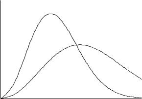
where v ¼ v2x þ v2y þ v2z . These lead to the familiar speed distribution curves like those in Fig. 1-7. Unlike the velocity vector, which can be negative, speed v is a scalar and is always positive. The probability of finding vx between the limits [a, b] is

pðvxÞ ¼	ða	FðvxÞdvx	ð1-26Þ
	b

20	COMPUTATIONAL CHEMISTRY USING THE PC

Probability Density

T = 200 K

T = 500 K

Speed

Figure 1-7 A Molecular Speed Distribution. The probability density is the expected number of speeds within an infinitesimal speed interval dv.

and the probability of finding v in the interval [a, b] is
pðvÞ ¼	ða GðvÞdv	ð1-27Þ
	b

The most probable value of the speed vmp can be obtained by differentiation of the distribution function and setting dGðvÞ=dv ¼ 0 (Kauzmann, 1966; Atkins 1990) to obtain

vmp ¼	m			ð1-28Þ
		2kBT		1=2

which is the particle speed at the peak of the curve in Fig. 1-7.

COMPUTER PROJECT 1- 4 j Maxwell–Boltzmann Distribution Laws

In chemical kinetics, it is often important to know the proportion of particles with a velocity that exceeds a selected velocity v0. According to collision theories of chemical kinetics, particles with a speed in excess of v0 are energetic enough to react and those with a speed less than v0 are not. The probability of finding a particle with a speed from 0 to v0 is the integral of the distribution function over that interval

ð0	GðvÞdv ¼ 2pkBT			ð0	eð mv =2kBTÞ4pv2dv	ð1-29Þ
v0		m	3=2	v0	2

ITERATIVE METHODS

21

The probability of finding a particle with a molecular speed somewhere between 0 and 1 is 1.0 because negative molecular speeds are impossible; hence, the relative frequency of speeds in excess of v0 is 1:0 Ð0v0 GðvÞdv.

It is convenient to reason in terms of the fraction of particles having a velocity in excess of vmp. The most probable velocity works as a normalizing factor, permitting us to generate one curve that pertains to all gases rather than having a different curve for each molecular weight and temperature. The integral of GðvÞdv over an arbitrary interval, however, cannot be obtained in closed form. It is usually integrated by parts (Levine, 1989) with the use of a scaling factor, to yield a three-term equation that is evaluated to give the fraction f ðvÞ of particles with speeds in excess of v0=vmp as a function of v0=vmp. This technique does not really escape the problem of nonintegrable functions because the second term in the evaluation for the frequency factor is a nonintegrable Gaussian.

It is also possible to integrate Eq. (1-29) directly by numerical means and to subtract the result from 1.0 to obtain the proportion of particles with speeds in excess of v0=vmp. In this project we shall use numerical integration of GðvÞdv

over

various

intervals to

obtain

f

ð

v

Þ

as a function of v0=vmp. Because

vmp

¼

ð

2k

B

T

=v0

Þ

[Eq. (14

Ð0 2

ð

Þ

2

m

1=2

-28)],

v0

G v

dv can be written

ð0

GðvÞdv ¼ pp X2e X dX ¼ 2:25626X2e X dX

ð1-30Þ

where X

¼

v

0=vmp.

This is the function we shall integrate in this project.

Procedure. Modify Program QSIM by substituting

DEF fna (X) ¼ X * X * EXP(-X * X) * 2.25626 in place of the DEF fna line of Program QSIM and put

(1-a) in place of

a

in the last line.

a.Using Program QSIM, generate the fraction of particles f(v) with a speed in excess of v0=vmp as a function of v0=vmp by numerical evaluation of the integral for intervals from 0 to 0.2, 0.4, etc. up to 2.0. Compare your plot of f(v) vs. v0=vmp with the literature (Kauzmann, 1966, Rogers and Gratzer, 1984).

b.Find the speed below which 75% of N2 molecules move at 500 K. On average, one in four N2 molecules is moving faster than the calculated value of v0 at 500 K. Why is f(v) near but not equal to 0.5000 when v0 ¼ vmp? The median speed is that speed at which half the particles in a collection are gong faster than vmed and half are going slower. Use Program QSIM to determine the ratio of vmed to vmp.

Because the computer cannot store an infinite number of bits, computations leading to very small and very large numbers are often inaccurate unless special

22	COMPUTATIONAL CHEMISTRY USING THE PC

precautions are taken. Results of the present calculation are poor at high velocities because of limitations imposed on handling very small exponential numbers.

Fortunately, an approximation formula for v0 1:0 is known (Kauzmann, 1966)

vmp

f ðvÞ ¼	pp e v		2v þ v	ð1-31Þ
	1	2	1

for the fraction of molecular velocities that are substantially in excess of vmp. Particles moving with these extreme velocities are rare but important because, in many reactions, only very fast-moving molecules react. The proportion of very energetic molecules relative to ordinary molecules, say those with speeds in excess of 4vmp, increases rapidly with temperature. This is the cause of an exponential rise of reaction rate with temperature observed in many reactions (Arrhenius’ rate law).

Atomic Orbitals

Once a numerical integration scheme that permits easy insertion of defined functions and convenient setting of the limits of integration has been set up and debugged, we may wish to use numerical integration for convenience rather than necessity. For example, establishing that hydrogenic wave functions have been correctly normalized and distinguishing between normalized and nonnormalized wave functions are common exercises in introductory quantum mechanic courses and can be mathematically difficult for all but the lowest atomic orbitals. Because the square of the wave function c2 at r is proportional to the probability of finding an electron within an infinitesimal interval r þ dr, the integral over the entire range 0 < r < 1 must be a certainty, pðrÞ ¼ 1:0.

Normalization is the process of finding a multiplicative constant for the wave function such that the integral of c2 over all space is 1.0. ‘‘All space’’ in this calculation is nonnegative because r cannot be less than 0.

The 1s orbital c1s ¼ e r is correct but not normalized. The normalized function governing the probability of finding an electron at some distance r along a fixed axis measured from the nucleus in units of the Bohr radius a0 ¼ 5:292 10 11 m is

c1s ¼ pp	a0 e r=a0	ð1-32Þ
1	1

The probability function (1-33 below) governs the probability of finding the electron at some distance r from the nucleus in any direction. Owing to the factor r2, this function gives us the probability of finding the electron anywhere within the interval r þ dr on the surface of a sphere of radius r. The radial function (1-32) is monotonically decreasing, but the function in spherical polar coordinates [Eq. (1-33)] goes through a maximum similar to that of the Maxwell–Boltzmann function of the last computer project.

Spherically symmetric (radial) wave functions depend only on the radial distance r between the nucleus and the electron. They are the 1s, 2s, 3s . . . orbitals