15

Modeling Catalytic Naphtha Reforming

Temperature Profile Selection and Benzene

Reduction

Rafael Larraz* and Raimundo Arvelo

University of La Laguna

Laguna, Spain

1INTRODUCTION

In 1952 CEPSA became the first European company to license UOP Platforming at its refinery on Tenerife [1]. Many things have changed since those days, but catalytic reforming of naphtha remains one of the major processes used at refineries, with the aim of increasing the octane number of naphtha or producing aromatics. Several of the reactions in the reformer, including naphthene dehydrogenation and cracking, also produce a high hydrogen content gas useful in middle distillate hydrotreating. The reformer unit is an integral part of the overall refinery or aromatics plant flow scheme and is a key contributor to profit generation.

Semiregenerative reformers typically consist of three or four adiabatic reactors loaded with a binfunctional catalyst. Reforming reactors operate at temperatures between 4608C and 5408C, and at a total pressure between 7 and 40 bar and with molar H2/hydrocarbon ratios between 3 and 8 [2]. High H2/ hydrocarbon ratios minimize coke deposition over the catalyst. Coke deposition decreases naphtha reforming activity and shortens the run length depending on operational severity. The reformer can be optimized for product quality, product yield, and catalyst cycle life by changing the operating variables, of which the

*Current affiliation: CEPSA, Madrid, Spain

551

552	Larraz and Arvelo

reactor inlet temperatures are the most widely used. The values of reactor inlet temperatures are known as the reactor temperature profile. The profile is characterized as flat if all temperatures are equal, ascending if temperature increases from the first reactor to the last, or descending if they decrease. The establishment of operational rules based on reformer operating variables helps the operating staff to improve unit yields.

Models are powerful tools, but the user has to be aware that sometimes the model does not match the plant which it is sought to simulate. Understanding the reasons can assist in using the model to the maximum of its capabilities. The reasons why simulations do not match the plant fall into three main categories [3]: (1) simulation effects or inherent errors, (2) sampling and analysis effects or measurement errors, and (3) model misapplication effects. A model must predict behavior not only within the reactor but in the auxiliary areas of the unit as well. It should also consider the complex nature of the process and the reaction that takes place during the process of reforming. Turpin [2] has given a detailed outline of the steps in catalytic reforming modeling, including the definition of the modeling objective, process identification, model selection, data collection and validation, and, finally, model calibration and verification.

The objective of this chapter is to outline a model for catalytic naphtha reforming [4,5] that can provide operational rules. The model also simulates how feed composition and operating conditions affect product compositions and yields. In addition, as practical applications of the model, a procedure for reactor temperature profile optimization is presented, as are some guidelines for improving reforming performance. Finally, an important issue for refiners, namely, reformate benzene reduction, is studied from the operational point of view.

The reforming unit model comprises a series of modules. One module covers feed composition calculation and a second is the naphtha reforming kinetic model where important issues such as reaction mechanism, reactor model, and flash drum calculations are discussed. A survey of thermodynamic equilibrium calculations is also made. A visually oriented development software (Microsoft VBA) has been used in model development allowing a user-friendly interface. The main screen snapshot is shown in Figure 1, along with the process flow diagram of the reformer modeled in this work.

2REFORMING THERMODYNAMIC EQUILIBRIUM CALCULATIONS

Equilibrium compositions are not usually attained under reformer operation conditions with the exception of naphthenes. But the knowledge of the reaction equilibrium values for C6 through C10 hydrocarbons provides upper bounds on

Modeling Catalytic Naphtha Reforming

553

Figure 1 Reforming model main screen snapshot.

actual aromatic and individual component yields. From the information cited in [6], a number of significant results are obtained:

For all carbon numbers, equilibrium aromatics decrease with decreasing temperature and increasing hydrogen pressures.

Even at high temperatures and low hydrogen partial pressures, equilibrium aromatics are low for C6 and C7 hydrocarbons; the effect is more pronounced at higher pressures. At high hydrogen pressures, this phenomenon is also found for the C8 and C9 hydrocarbons, where aromatic formation is no longer quite as favorable as at low hydrogen pressures.

For all temperatures, hydrogen pressures, and carbon numbers, both alkylcyclohexanes and alkylcyclopentanes are essentially absent from the equilibrium mixture.

For all temperatures, hydrogen pressures, and carbon numbers, the equilibrium favors isoparaffins over normal paraffins.

The availability of an equilibrium calculation procedure gives a deep insight into the behavior of reforming reactions. Some thermodynamic equilibrium calculation procedures are discussed in the following sections.

554	Larraz and Arvelo

2.1.Rigorous Methodology

A free-energy minimization method is used to determine equilibrium chemical composition of the gaseous mixture at constant temperature and pressure. The free total energy of the system is minimized by means of the free molar energy of each species, thus maintaining the number of atoms of each element. Considering a reaction or system of reactions producing products from different reactants, the equilibrium conversion of each species is obtained by minimizing the expression

Gðn1; n2; . . . ; nNÞ ¼ Snj½ðDGTÞj=RT þ lnðnj PÞ&

ð1Þ

subject to the mass balance constraints:

Saij nj ¼ bi ði ¼ 1; 2; . . . ; mÞ;

nj 0 for 8j

ð2Þ

where G is the total Gibbs free energy of the system, P is the total pressure, T is the temperature, R is the universal gas constant, D(GT)j is the free energy of formation at temperature T(K) for the species j defined from its constituent elements in their reference states, cal/mol; bi is the total sum of atom-gram or mol-gram of element i present in the reactants, and, aij is the number of atoms of element i of the reactants present in the products j. Correlation to obtain the free energy of formation, DGf, for the main components of naphtha has been compiled and expressed as a function of the temperature using the following equation [7]:

DGf ¼ A þ BT þ CT2	ð3Þ
The linear mass balance, Eq. (2), becomes [8]:
2n1 þ m2n2 þ þ mnnn ¼ b1	ð4Þ
c1n1 þ c2n2 þ þ cnnm ¼ b2	ð5Þ

Equation (4) is a hydrogen balance with mi the number of hydrogen atoms in species i; Eq. (5) is a carbon balance with ci the number of carbon atoms in species i. The ratio b1/b2 is the hydrogen-to-carbon ratio in the mixture.

Hydrogen partial pressure has an extremely important effect on process yields and on the rate of catalyst deactivation. Consequently, each catalyst is designed to operate at specific hydrogen pressures. Therefore, it is desirable to report the results of the idealized equilibrium calculations at constant hydrogen partial pressure so that they may be compared to actual process data.

The equilibrium compositions are determined without knowledge of the specific chemical reactions involved [9]. Due to the fact that the function described in Eq. (1) is convex, the conjugate gradient algorithm is ideally suited to solve this problem [10]. In carrying out the equilibrium calculation, care must be taken to ensure nontrivial results. Because hydrocracking reactions are the most energetically favorable reactions [11], the equilibrium compositions are

Modeling Catalytic Naphtha Reforming

555

calculated separately for hydrocarbon mixtures of the same carbon number. The equilibrium results are thus idealized because they are applicable only in the absence of cracking.

2.2.Shortcut Method

When it is necessary to estimate the equilibrium composition of the many complex reactions that occur during catalytic reforming of naphtha, a simple and precise method could be employed [12]. The method uses individual equilibrium compositions to derive generalized equilibrium constants for each carbon number group from six carbons up to nine carbons. This method assumes that paraffins do not change their carbon number when converted to aromatics during the catalytic reforming process. As previously, hydrocracking reactions are neglected. It is also assumed the reformate naphthenes content remains low. The key reaction of catalytic reforming, dehydrocyclization, converts paraffins to aromatics:

Pi , Ai þ 4H2

i ¼ 6; 7; 8; 9

The equilibrium constant for this reaction is

Ki;P ¼ ðxi;A=xi;PÞpH2 4

ð6Þ

where

Ki,P ¼ equilibrium constant for the paraffins in the y carbon number group xi,A ¼ aromatic content of the y carbon group, mole fraction of the total

mixture

xi,P ¼ paraffin content of the y carbon group, mole fraction of the total mixture

pH2 ¼ hydrogen partial pressure, atm

If we let B symbolize the mole fraction of each carbon number group based on the total moles of the mixture, the material balance is:

9	Bi ¼ 1			ð7Þ
i 6
¼
Since naphthenes are assumed zero
Pi ¼ xi;A þ xi;P		and	xi;P ¼ Bi xi;A	ð8Þ

Including this expression to the equilibrium constant equation and rearranging terms, we obtain:

xi;A ¼ ½Ki;P=ð pH2 4 þ Ki;PÞ&Bi

ð9Þ

556	Larraz and Arvelo

Table 1 Dehydrocylization

Equilibrium Constant Coefficients

(ln K ¼ að103=TÞ þ b. Range 650–

829 K)

Carbon number	a	b
C6	232.6	51.17
C7	231.24	53.36
C8	229.70	53.36
C9	228.94	53.78

Source: Ref. 12.

The total aromatic concentration of the mixture is shown by the following

xi;A ¼	9		6 xi;A ¼	9	½Ki;P=ð pH2	4	þ Ki;PÞ&Bi	ð10Þ
	i	¼		i 6
				¼

The total paraffin concentration is found by the difference with the mole fraction of each carbon number group Bi.

The equilibrium constants for each hydrocarbon type are given in Table 1, reporting temperature effects as an integrated form of the Van’t Hoff equation. These data were obtained by means of equilibrium calculations of a mixture of 104 components including hydrogen. Free-energy minimization techniques were employed and substitution of the equilibrium composition for each carbon number group in the mass balance equation provides the specific equilibrium constants Ki,P.

The procedure includes some corrections in order to account for the cracking reactions, which occur during the reforming reactions. Cracking tends to increase the composition of the C6 and C7 hydrocarbons in the product, while the composition of the C8 and C9 hydrocarbons is decreased. Table 2 presents calculation results for two different operating conditions.

3FEED CHARACTERIZATION TECHNIQUE

Advanced control strategies and optimization techniques are frequently applied to catalytic reforming in order to obtain greater economical benefits and ease unit operations. The basis for success of these strategies and techniques is the availability of on-line feed and product quality measurements. These are further described in Chapter 14. The traditional approaches employed tend to be on-line analyzers and algorithms based on quick analyses of density or distillation performed in situ. In order to obtain reformer feed composition on-line and

Modeling Catalytic Naphtha Reforming					557
Table 2 Equilibrium Concentration of Aromatics
		Feed composition
B6	Bi ¼ xi;A þ xi;P; i ¼ 6; . . . ; 9=SBi9¼6 ¼ 1
		B7		B8	B9
0.24		0.30		0.28	0.18
		Results
T/P		T ¼ 482/5308C, P ¼ 10/30 kg/cm2
	x6,A	x7,A	x8,A	x9,A	xA
482/10	0.103	0.281	0.278	0.180	0.842
482/30	0.004	0.069	0.216	0.163	0.452
530/10	0.225	0.299	0.280	0.180	0.984
530/30	0.054	0.250	0.275	0.179	0.785

Source: Ref. 12.

without time delay, an estimative naphtha characterization algorithm based on the correlation of physical properties is presented and a relatively new methodology for naphtha characterization, known as nuclear magnetic resonance (NMR), is described in brief.

3.1.Feed Characterization Algorithm

The naphtha used as catalytic reformer feedstock usually contains a mixture of paraffins, naphthenes, and aromatics in the carbon number range C5 to C10. The analysis of feed naphtha is typically reported in terms of its American Society for Testing and Materials (ASTM) distillation curve and API gravity. Since reforming reactions are described in terms of lumped chemical species, a feed characterization technique based on the correlation of physical properties with reformate boiling range and density has been implemented by Taskar and Riggs [13] in naphtha reforming modeling of industrial units. Several other methods based on neural networks exist in the literature that allow feed composition in terms of paraffins, olefins, naphtenes, and aromatics (PONA) and reformate octane number prediction [14,15]. The proposed method results exhibit errors ranging from 3% to 10%. The main steps of the procedure are described below.

The ASTM distillation data are first converted to true boiling point data. Riazi et al. [16] compile experimental data on ASTM, TBP, and EFV distillation of fractions from different sources. Using this set of data, the following equation was found to be the simple form for interconversion of distillation data.

t ¼ aubSc

ð11Þ

558 Larraz and Arvelo

where t (TBP or EFV) and u (ASTM) are temperatures (in 8R) at the same vol % vaporized, S is the specific gravity, and a, b, and c are constants. If the specific gravity is not known, Eq. (12) could be used with an average deviation of about 2%.

S ¼ at10 bt50 c

ð12Þ

where t10 and t50 (8R) are temperature at 10% and 50% in ASTM, TBP, or EFV curve. The TBP curve is decomposed into a number of discrete volume fractions. According to Lion and Edmister [17], the specific gravity of each volume fraction is evaluated assuming constant UOP characterization factors.

Riazi et al. [18] have given a correlation table to predict physical properties of hydrocarbon mixtures using average boiling point and specific gravity in an

empirical equation of the form	ð13Þ
P ¼ aTbSc

where P is a physical property to be predicted, T is the average boiling point in 8R, and S is the specific gravity at 608F. Constants a, b, and c are shown in Table 3 for different physical properties. Prediction accuracy is reasonable, and average deviations remain under 3.5% over the boiling range of 40–4508C for the following properties: molecular weight, liquid density, liquid molar volume, critical temperature, critical pressure, critical volume, refractive index, heat of vaponzation, and ideal gas heat capacity. Since the materials boil over a range of temperatures, any one average boiling point fails to correlate all of the properties. In general, the average boiling points listed are used for estimating the physical properties:

Volume average boiling point Molal average boiling point Mean average boiling point

Specific heat Pseudo-critical temperature Pseudo-critical pressure Molecular weight

Heat of vaporization Density

Liquid molar volume

Table 3 Correlation Constants for Equation P ¼ aTb bSc

Property	A	b	c
Mol. wt	4.5673E-3	2.1962	21.0164
Critical temp. (8R)	24.2787	0.58848	0.3596
Critical pressure (psia)	3.12281E-9	22.3125	2.3201
Molar volume at 208C (cm3/gmol)	7.6211E-5	2.1262	21.8688
Density (g/cm3)	0.982554	0.002016	1.0055
Heat of vaporizat. (Btu/lb mol)	8.48585	1.1347	0.0214
Specific heat at 08F (Btu/lb mol)	4.0394E-7	2.6724	22.363

P, physical property; Tb, normal boiling point (8R); S, specific gravity.

Source: Ref. 16.

Modeling Catalytic Naphtha Reforming

559

Each TBP fraction is composed of a mixture of chemical species whose boiling points fall within the TBP range of the corresponding fraction. An adaptive random search (ARS) algorithm [19–22] is applied in order to find the naphtha chemical composition, in terms of paraffins, naphthenes, and aromatics, that provides the best match between predicted and observed physical properties in each volume fraction. The entire mixture composition is then calculated from the volume fractions. Olefin species are not considered, introducing an error of about 0.5% into the naphtha composition. Pure hydrocarbon properties have been extracted from the API tables [23].

The composition of a naphtha reforming feed is studied employing the outlined characterization method. Specific gravity and ASTM D86 distillation of reforming feed are used as source data, then a split into discrete fractions with gravity assay estimations is made, as shown in Tables 4 and 5. Density and molecular weight are the physical properties that have to be adjusted. Table 6 gives the predicted values for each fraction of feed naphtha. The adjusted composition of the naphtha feed is presented in Table 7, detailing each fraction composition. Assay needs are limited to a D86 ASTM and an API or specific gravity; and even this information could be avoided employing Eq. (12). Method error varies from 3% to 10% but gives enough information to predict feed quality changes and to monitor unit performance.

3.2.NMR On-line Analyzers

During an NMR analysis, a sample stream is passed through a precisely controlled magnetic field. The protons of the sample ‘line up’ with the homogeneous magnetic field. To take a reading, the NMR analyzer transmits

Table 4 Reformer Naphtha Feed

Assay

Assay (vol %)	Naphtha feed (8C)
ASTM 0%	105
ASTM 10%	114
ASTM 30%	122
ASTM 50%	131
ASTM 70%	147
ASTM 90%	168
ASTM 95%	182
ASTM 100%	200
RON	39.5
SPGR at 158C	0.7471

560	Larraz and Arvelo

Table 5 Distillation Ranges and Density

Estimation Naphtha Feed

Fraction (8C)			Vol %	Density (KUOP)
10	–40
40	–70
70	–100		21.0	0.703
100		–125	22.0	0.737
125		–150	26.0	0.755
150		–175	20.0	0.769
175		–EP	11.0	0.787
IP–EP			100.0	0.7471a

Table 6 Estimated Properties Naphtha Feed

			Molecular weight
Fraction (8C)		Density (P/N/A)	(P/N/A)
10	–40
40	–70
70	–100	0.684/0.756/0.878	96/89/80
100	–125	0.702/0.770/0.866	112/102/94
125	–150	0.717/0.779/0.865	129/115/104
150	–175	0.730/0.793/0.865	145/130/120
175	–EP	0.750/0.800/0.870	160/150/135

Table 7 Calculation Results

Fraction (8C)		Naphtha feed (P/N/A) (vol %)
10	–40
40	–70
70	–100	85.2/13.1/1.7
100	–125	59.0/30.7/10.5
125	–150	53.3/29.9/16.8
150	–175	55.3/28.5/16.2
175	–EP	53.2/27.1/19.7
IP–EP		62.5/25.6/11.9

Modeling Catalytic Naphtha Reforming

561

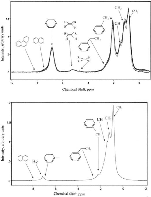
pulses of radiofrequency energy into the stream, which deflects the protons off their aligned axis. The amount of deflection and the subsequent recovery time vary according to molecular structure, and the NMR analyzer reads this structure by analyzing frequency signals emitted by the spinning protons. The analyzer averages multiple pulses into a spectrum that reveals chemical species and their concentrations. This spectrum can then be correlated with physical properties in addition to the chemical composition, enabling determination of multiple parameters in a single spectrum. And since NMR is not an optical technology, the analysis is essentially independent of sample state or physical condition. In NMR spectroscopy, the surrounding molecular structure determines where the species will be resolved in the spectrum. These peaks occur at known positions, and their intensity is directly proportional to concentration. These facts contribute to the high precision and accuracy of the NMR method.

In Figure 2 several groups of spectra showing different naphtha streams and the chemical makeup of the streams as observed by NMR are presented. The aromatic, olefinic, and aliphatic regions are in their own distinct areas of the spectrum. Different types of olefins can be quantified, i.e., terminal vs. internal olefin, as well as trisubstituted, disubstituted, and vinylidene olefin distributions. Monoaromatics are readily discerned from PNAs, and benzene is observed as a single resonance. The aliphatic protons are observed as peaks due to CH3, CH2, and CH proton types. This yields direct information about branching character and linear character, i.e., paraffin vs. isoparaffin content. The chemical detail that NMR provides will not only allow correlation to PONA-type analyses but also allow speciation of olefinic and aromatic types. In Table 8 a statistical analysis is presented [24]. This extremely precise analysis allows kinetic model parameter correlation to be made frequently and on-line.

4NAPHTHA REFORMING KINETIC MODEL

From a fundamental point of view, kinetics contributes to a better understanding of the reaction mechanisms and of the effect of catalysts on these. From a practical point of view, accurate kinetic equations are of great importance for the reliable design and simulation of the reactors. Relatively few reaction models of the reforming process have been suggested in the literature pertaining to this field. The first significant attempt at delumping naphtha into different constituents [25] considered naphtha to consist of three basic components: paraffins, naphthenes, and aromatics. Due to its simplicity, this model is still used. Basing his work on Smith’s model, Barreto et al. [27] included certain modifications concerning discrimination between the reaction rates for aromatization of fiveand six-ring naphthenes, the consideration of two kinds of paraffins with different reactivities, and the inclusion of an overall hydrodealkylation reaction. Also

562	Larraz and Arvelo

Figure 2 Naphtha composition by NMR. (a) Heavy Cat–cracked naphtha. (b) Straightrun naphtha.

Modeling Catalytic Naphtha Reforming				563
Table 8 On-line Comparison of I/A Series Process NMR and Laboratory GC Analysis
	Mean conc.	Mean dev.	Std. dev.	Correlation
Parameter	(wt %)	(wt %)	(wt %)	coefficient
Total normal paraffin	34.10	20.15	0.78	0.980
Total isoparaffin	32.01	0.01	0.66	0.975
Total naphthenes	20.40	0.04	0.63	0.983
Benzene	1.99	0.01	0.11	0.993
Toluene	1.99	20.01	0.15	0.995
Ethylbenzene	0.33	0.00	0.04	0.993
Xylenes	1.56	0.01	0.08	0.999
C9 Aromatics	0.65	0.01	0.12	0.993
C10 Aromatics	0.14	0.01	0.06	0.962
Total aromatics	6.66	0.01	0.17	0.999

Source: Ref. 24.

based on Smith’s model, Ansari and Tade [28] developed a multivariate control application after testing it against existing plant data. In a more extensive attempt to model reforming reactions of whole naphtha, Krane et al. [29] recognized the presence of various carbon numbers from C6 to C10 as well as the difference between paraffins, naphthenes, and aromatics within each carbon number group. The model derived by Krane contained a reaction network of 20 different components. An improved model has been proposed by Aguilar and Anchyeta [30,31] where the Krane model is modified to account for temperature and pressure variations. Burnett [32] proposed a similar model. Jenkins and Stephens [33] employed first order rate equations including reversible ones to develop a kinetic model, the effect of pressure on the reaction rate is simulated by means of a pressure factor with a characteristic exponent for each particular reaction. The first mention of a different treatment for the C5 and C6 ring naphthenes was made by Henningsen and Bundgaard-Nielson [34] who also gave accurate values for the heat of reaction and activation energies of the reactions involved in the model.

All the models described were pseudo-homogeneous in nature. Kmak [35] presented the first model incorporating the catalytic nature of the reactions by deriving a reaction scheme with Hougen–Watson–Langmuir–Hinshelwood– type kinetics. Rate equations derived from this type explicitly account for the interaction of chemical species with the catalyst. In another notable effort, Ramage et al. [36] developed a detailed kinetic model based on extensive studies of an industrial pilot plant reactor. The model accurately simulates commercial reactor performance and has been applied routinely in Mobil refineries under the name of KINPTR [37]. New continuous regeneration reforming units have been simulated by Lee et al. [38], and Taskar has employed a rigorous kinetic model to

564	Larraz and Arvelo

optimize performance in an industrial reformer by studying operating modes and the influence of operational variables [13].

The Kmak model was later refined by Marin and coworkers [39], who presented the reaction network for the whole naphtha. Containing hydrocarbons in the carbon number fraction from C5 to C10, the reaction network included 23 pseudocomponents and used Hougen–Watson rate equations. Marin and Froment [40] and Van Trimpont et al. [41] also conducted separate studies on C6 and C7 carbon number fractions, respectively, and developed the corresponding Hougen–Watson rate equations. Various possible reaction paths and mechanisms were systematically evaluated before choosing the one that best fits the experimental data provided by a laboratory scale reactor. An extensive experimental program with various feeds led to a plausible reaction mechanism using kinetics of the Hougen–Watson type [39,42]. The reaction network involves hydrogen and 92 hydrocarbons ranging from C1 to C11, including all individual detectable hydrocarbons up to and including C8. Between certain hydrocarbons, equilibrium is reached so that lumping is permitted. This leads to 29 lumps: hydrogen, methane, ethane, propane, butanes, pentanes, multibranched hexanes, single-branched hexanes, n-hexane, five-ring naphthenes, benzene, sixring naphthenes, the analogues of the C6 lumps for C7 and for C8 separately, and, finally, five C5þ lumps involving C9 to C11 hydrocarbons divided into isoparaffins, n-paraffins, five-ring naphthenes, six-ring naphthenes, and aromatics [43]. This definitive model has been extended as a collaboration between IFP and Froment’s group, in order to cover reformer units dynamic simulations thus providing an operator training tool as well as unit performance monitoring [44].

Diffusional effects in naphtha reforming modeling are not usually treated separately. The uncertainty associated with diffusion effects in the catalyst pellets is lumped into the kinetic rate parameters [13,39]. If there are diffusional limitations inside catalyst pellets, the effective reaction rates differ from the intrinsic reaction rates at surface conditions. To solve the problem the preexponential factor in the rate equation is tuned as an adjustable parameter matching simulation results to reality. Coppens and Froment [43] improved reforming models by including diffusional effects into rate equations. Inside catalyst pellets, diffusion and reaction is described by the continuity equations for the M lumps:

r Nj ¼ rsRj

j ¼ 1; . . . ; M

ð15Þ

together with Stefan–Maxwell flux equations for multicomponent diffusion [45]:

100=RTrpj ¼	M	ð pkNj pjNkÞ=ð ptDe;jkÞ ¼ Nj=De;jk
	k¼1
j ¼ 1; ; M		ð16Þ

Modeling Catalytic Naphtha Reforming

565

In their model, the porous nature of the reforming catalyst support (g-alumina) is approximated by a self-similar fractal structure (see Appendix at the end of the chapter). Fractal dimension, D, of the catalyst is obtained by means of smallangle X-ray scattering (SAXS) and expressions for Knudsen diffusion in terms of fractal dimension are provided [46–49]. Model results showed that the effects of the total fractal surface morphology on the product distribution and yields are significant. When the intrinsic reaction rates per unit catalyst mass are the same, a catalyst with a smooth surface, D ¼ 2, yields 18.9 wt % isoparaffins and 70.1 wt % aromatics while a catalyst with a fractal surface, D ¼ 3, yields 21.7 wt % isoparaffins and 66.2 wt % aromatics. This is a result of the stronger diffusional limitations found within catalysts with a fractal surface, as compared to catalysts with a smooth surface.

4.1.Reaction Mechanism

As reaction kinetics play a paramount role in catalytic reforming model performance we have employed a rigorous model [36,39] in our calculations. The naphtha used as catalytic reformer feedstock contains a mixture of more than 285 different chemical species, mainly paraffins, naphthenes, and aromatics in the carbon number range C5 to C10. This overwhelming number of chemical components requires chemical component lumping into a smaller set of kinetic lumps [50] to make the reforming reactions network tractable. Naphtha reactions in catalytic reforming are dehydrogenation of naphthenes, isomerization of paraffins and naphthenes, dehydrocyclization of paraffins, and hydrocracking of paraffins. The selectivity changes considerably between six-carbon, sevencarbon, and eight-carbon species in a given molecular class. For hydrocarbons containing eight or more carbon atoms the selectivity within a molecular class does not vary significantly due to the similarity of their aromatization equilibrium data [6]. Therefore, the C6, C7, and C8þ lumps are considered plus a total C52 lump. The reaction network and lumping scheme are shown in Figure 3.

Due to recent legislation reformate benzene content has been limited, and knowledge of the benzene formation mechanism could be an aid to finding procedures that ease the task of meeting the new specifications. The first sources of benzene in reformate that can be identified are benzene and benzene precursors from the C6 fraction of the feed. As a result of the benzene formation mechanism [40], it can be expected that cyclohexane from the feed is almost completely dehydrogenated into benzene. To convert methylcyclopentane to benzene is much more difficult because methylcyclopentane first has to be converted into cyclohexane by functional dehydrogenation and a ring isomerization reaction. Particularly in the case of methylcyclopentane, ring isomerization is a difficult step since a more stable secondary methylcyclopentane carbenium ion has to be isomerized into a less stable primary cyclohexane carbenium ion. Nevertheless,

566	Larraz and Arvelo

Figure 3 Lumping scheme reaction network.

once the cyclohexane intermediate is formed, it is easily dehydrogenated to benzene. Finally, the aromatization of n-hexane is even more difficult because n- hexane must be converted to cyclic compounds by slow dehydrocyclization reactions. As a rule of thumb it can be said that only about 20 wt % of n-hexane and 50 wt % of methylcyclopentane from the feed are converted into benzene [51]. Next to benzene precursors from the C6 fraction of the feed, hydrocracking of higher molecular weight hydrocarbon fractions can form benzene precursors. C7þ aromatic compounds can be dealkylated, which also can lead to the formation of benzene. A differentiation is made between C6, C7, and C8þ compounds only. This is justified by the fact that in general the aromatization selectivity of paraffins and cyclopentanes increases with chain length. However, the differences in selectivity between C8þ compounds are very small. An increase in the selectivity for hydrocracking reactions may lead to a higher benzene content of the reformate [52]. Reforming catalysts are generally known as bifunctional catalysts because the metallic and the acid sites are discrete components. They cooperate in promoting the desired overall reactions, but each appears to be responsible for certain steps. The two functions of a reforming catalyst—metallic and acid—are balanced carefully for reaction conditions. If the balance is shifted, side reactions occur. Benzene selectivity is enhanced with

Modeling Catalytic Naphtha Reforming

567

high acidity catalyst as the C8þ aromatics selectivity is decreased [52]. So the catalyst chloride level has to be strictly controlled in order to avoid benzene formation due to a strong acid function.

4.2Reactor Model

Simulation of reforming reactors which incorporates the kinetic model has been made according to the following procedure. The mass, energy, and momentum equations for an axial flow reactor are:

	dF=dz ¼ rbVR				NC				ð17Þ
	dT=dz ¼ rbMm=ðGcpÞ					ð DH0 f ÞjRj			ð18Þ
					j¼1
	dp	=dz	¼	1:5 10 3ð1 1Þ2mG				1:75 10 5ð1 1ÞG2	ð	19	Þ
	t			13pf ðdpÞ2				13pf dp

Initial conditions are F ¼ Fo, T ¼ To, and pt ¼ pto at z ¼ 0. The production rates Rj are obtained from:

Rj ¼ Sbijri

j ¼ 1; . . . ; Nc

ð20Þ

bij is negative for reactants and positive for products of the single reaction i. The rate expressions of the individual reactions, ri, are of the Hougen–Watson type and are shown in Table 9. For the dehydrogenation of six-ring naphthenes a firstorder rate expression is used. The dehydrogenation is much faster than the former reactions and is diffusion limited, and this criteria is analogous to the approach of Marin et al. [39]. The activation energies and pre-exponential factors used are shown in Table 10 as well as the reaction heats involved. Gear’s numerical integration scheme for solving stiff ordinary differential equations was employed to integrate the equations through each fixed-bed reactor. Figure 4 presents the calculation sequence, including flash drum calculations.

Table 9 Catalytic Reforming Reaction Rate Expressions

Hydrocracking	rHydrocracking ¼ Ae E=RTðPAPHÞ=G
Isomerization	rIsomerization ¼ Ae E=RTðPA PB=KABÞ=G
Dehydrocyclization	rDehydrocyclization ¼ Ae E=RTðPAPBPH=KABÞ=G

A, pre-exponential factor; E, activation energy; G, adsorption term; H, hydrogen; A, reactant; B, product; KAB, equilibrium constant; Pi, partial pressure of component i.

568								Larraz and Arvelo
Table 10 Heats of Reaction (kcal/gmol)
	Reaction			C6	C7	C8		C9
	N6 , N5		3.8		4.5	7.1		8.8
	N6 þ H2 , P		210.6		28.4	27.3		25.8
	N5 þ H2 , P		214.4		213.0	214.4		214.6
	N6	, A þ 3H2	52.3		51.5	49.9		51.0
	N5	, A þ 3H2	48.5		47.0	42.8		42.2
	P , IP		22.3		22.3	21.9		22.0
	N6	þ H2 , IP	212.9		210.7	29.1		27.8
	N5	þ H2 , IP	216.7		215.2	216.2		216.6
			Kinetic Rate Equation Parameters
				Pre-exponential factor				Activation
								energy
						C8þ
Reaction				C6	C7			(cal/mol)
Hydrocracking			4.18 E12		1.61 E13	1.76 E13		53000
Dehydrocylization			1.0188 E11		1.37 E10	3.23 E10		45000
Dehydrogenation			1.35 E08		3.04 E08	7.24 E08		30000
Isomerization			7.72 E07		3.08 E08	3.25 E08		40000

Source: Ref. 6.

Deactivation Function

Coke deposition causes deactivation of the catalyst, resulting in a reduction of the reforming reaction rates. Coke is generated from the olefinic intermediates formed during the course of the main reforming reactions. Higher hydrogen pressures suppress the diolefin formation, thereby reducing coke formation [54]. As has been confirmed experimentally by means of temperature-programmed oxidation tests, deactivation during the first hours of the run is due to coke deposition on the metal and thereafter to deposition on the support, which produces minor deactivation [55,56]. Catalyst deactivation can be accounted for by introducing a deactivation function [40,57] f for each of the so-called main reactions:

ri ¼ ro if

0 , f , 1

ð21Þ

The deactivation function depends on catalyst coke content rather than run length as commonly considered. The dependence has the form

fi ¼ e aiCc

ð22Þ

Modeling Catalytic Naphtha Reforming

569

Figure 4 Model calculation flow chart.

570	Larraz and Arvelo

where fi is the deactivation function for reaction i, ai is the deactivation constant for reaction i, and Cc is the amount of coke over the catalyst. Coke production is obtained as a function of hydrogen partial pressure and aromatic production, and the expression used is based on the work of Schro¨der et al. [58] who found the following relationship for the coke formation where both a paraffinic and aromatic coke formation is assumed.

dC=dt ¼ ðkppp þ kApAÞpH2 n1Cn2f	ð23Þ
With n1, n2 , 0:
kp ¼ kp1 expð Ep=RTÞ	ð24Þ
kA ¼ kA1 expð EA=RTÞ	ð25Þ

Deactivation parameters are shown in Table 11 for each of the main reforming reactions as well as for the coking reaction.

Parameter Estimation

For specific rate constants and corresponding pre-exponential factor and activation energy, many of the data are available in literature. These data were used as preliminary values for model development. Unfortunately this approach does not necessarily describe the performance of commercial units; thus, a calibration procedure was implemented [59]. The parameter estimation procedure is presented in Figure 5. Activation energies were kept constant and a pre-exponential factor has been used as an adjustable parameter. The procedure assumes literature data for unknown constants. The resulting rate equations are numerically integrated using the inlet data from individual runs as initial conditions. The deviation is calculated by subtracting the computer-determined value from the observed value of all variables. The resulting deviations for that run are then added to the sum of deviations from all runs. This double summation of deviations is the objective function or criterion of the fit of the data to the

Table 11 Deactivation Parameters

	Activation energy (cal/mol)
Deactivation function	C6	C7	C8þ
kP (paraffinic)	49000	90000	90000
kA (aromatic)	14000	47000	47000

Source: Ref. 58.

Modeling Catalytic Naphtha Reforming

571

Figure 5 Parameter estimation procedure.

model. The constants are then varied one at a time to minimize this objective function, which is presented in Eq. (26):

Fð j; iÞ ¼ Sj¼1 jSi¼1 ikYj;i Yj;ik

ð26Þ

A conjugate gradient algorithm is used in the calculations, and different initial values have been tested in order to avoid local minimums.

5FLASH DRUM SEPARATOR MODEL

The flash drum separator, which separates the hydrogen and some lighter gases from heavier products, was modeled as an isothermal flash operation. Equilibrium is established between the vapor and liquid phase. The mass balances and vapor liquid equilibrium equations for component j of the stream are

572		Larraz and Arvelo
written as:
Ftzj ¼ Fvyj þ F1xj	j ¼ 1; . . . ; Nc	ð27Þ
Kj ¼ yj=xj	j ¼ 1; . . . ; Nc	ð28Þ

The conservation of total mass in the vapor and in the liquid phase is expressed by:

NC	NC	ð29Þ
j¼1 yj ¼ 1 and	j¼1 xj ¼ 1

The energy equation is written as:

Q ¼ HvFv þ ðH1F1 Hf FtÞ

ð30Þ

When composition and flow rate of the product stream fed to the flash drum as well as the temperature and pressure of the flash condensation are known, Eqs. (27) to (30) form a set of 2NCþ3 nonlinear algebraic equations that are solved by means of the Newton–Raphson algorithm. Since the product gas mainly contains components at conditions exceeding their critical point, nonideal behavior of the mixture is accounted for by calculating the vapor liquid distribution coefficients according to Chao and Seader [60]:

Kj ¼ Ojv=ðgj1Vj1Þ

ð31Þ

The vapor fugacity Ojv is obtained from the Redlichh–Kwong equation of state. The activity coefficient, gj1, is derived from the correlation of Flory and Huggins [61]. The recycle gas compressor is used to compensate for the pressure drop in the loop. The power consumption of the compressor could be estimated on the basis of calculated adiabatic head and flow rate of recycle gases:

DHadiabatic ¼ RTinletðk=k 1ÞfðPout=PinÞk 1=k 1g

ð32Þ

6MODEL APPLICATIONS

Catalytic reformers are designed with operational flexibility in mind, whether for motor fuel production or to produce aromatics such as benzene, toluene, and xylenes. The variables that affect the performance of the catalyst and change the yield and quality of reformate are feedstock properties, reaction temperature, space velocity, reaction pressure, and hydrogen-to-hydrocarbon ratio [62]. The reactor inlet temperatures are invariably the most effective tool at the refiner’s disposal to obtain the required reformate quality. As catalysts lose activity in operation, reactor temperature is gradually increased to maintain a constant octane number in the product reformate [63]. Since multiple factors affect

Modeling Catalytic Naphtha Reforming

573

reforming performance, a unit model appears as an useful tool to improve unit capabilities and extend cycle length. In the following sections, two important issues have been selected as reforming model applications. First, model performance against an industrial unit is outlined; then an analysis is made of reactor temperature profile influence over reforming performance and run length. Second, the effect of operational variables over benzene formation during naphtha reforming is studied, and some recommendations are made in order to reduce the reformate benzene content.

6.1.Reforming Model Performance

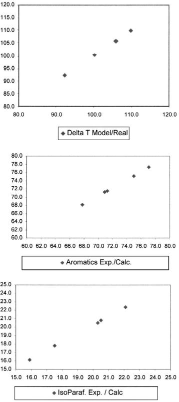
The reforming model described was used as a monitoring tool for an industrial semiregenerative reforming unit. The main operating parameters for the industrial reformer are presented in Table 12. The data employed were obtained from the control system and cover a 6-month period so catalyst deactivation could be evaluated. Reformate composition and reactor DT values were used to calibrate the model. Model fitting to plant data are shown in Figure 6, and model accuracy is satisfactory for the selected variables. Based on these results, one can expect a reasonable model predictive capability.

Catalyst deactivation was estimated using the deactivation function paradigm, and deactivation results for the main reforming reactions are presented in Figure 7. From the graphs obtained, a slight relative deactivation is observed for the aromatization, dehydrocyclization, and isomerization reactions ranging from 0.85 to 0.7. This supports the fact that the catalyst is still active and is at about midlife condition.

Table 12 Industrial Semiregenerative Reformer Operating Parameters

Date	31/10/2001 30/11/2001 30/12/2001 29/01/2002 26/02/2002
Flow rate (BPSD)	24034	25326	24985	25748	25867
Reactor temp.
1 Rx	519	521	522	523	524
2 Rx	511	514	515	516	517
3 Rx	511	514	515	516	517
Pressure (kg/cm2)	29	29	29.8	30	30
Feed composition
Paraffins	25.8	24.7	22.4	24.0	25.3
Isoparaffins	31.5	29.6	28.9	28.1	29.6
Naphthenes	31.8	34.8	37.4	37.7	34.5
Aromatics	10.8	10.6	10.3	10.0	10.5

574	Larraz and Arvelo

Figure 6 Comparison of industrial reformer data and model calculations for reactor DT, aromatics, isoparaffins, paraffins, and naphthenes.

Modeling Catalytic Naphtha Reforming

575

Figure 6 Continued.

Figure 7 Deactivation function evolution with time for reforming reactions.

576	Larraz and Arvelo

6.2.Naphtha Reforming Heat Needs

In a typical semiregenerative naphtha-reforming unit the reformer reactor charge is combined with a recycled gas stream containing 60–90 mol % hydrogen. The total reactor charge is first heated by exchange with effluent from the last reactor and then in the first charge heater. Radial reactors are commonly used to obtain low-pressure drops. The major reactions in the first reactor, such as naphthene dehydrogenation, are endothermic and very fast, causing a sharp temperature drop in the first reactor. For this reason, catalytic reformers are designed with multiple reactors and with heaters between the reactors to maintain reaction temperature at operation levels. The last reactor effluent is cooled by heat exchange with the reactor charge; then it enters the product separator where flash separation of hydrogen and light hydrocarbon takes place. The flashed vapor is compressed and sent to join the naphtha charge. Excess hydrogen from the separator is sent to other units in the refinery, such as diesel hydrotreating. The separator liquid is pumped to the reformate stabilizer and then the light hydrocarbons free reformate is sent to storage.

In the design of chemical reactors where two or three reactions are involved, the choice of the appropriate temperature is usually made by increasing or decreasing the reaction temperature depending on whether the activation energy of the desired reaction is higher or lower, respectively [64]. Catalytic reforming reactions have very similar activation energies, with the exception of coking which favors high temperatures. So this simple criterion is not valid. Reformer naphtha is composed of normal and branched paraffins, fiveand sixmembered ring naphthenes, and single-ring aromatics. Each of these general feed constituents can undergo several competing reactions during the various sections of the reaction as has been discussed in earlier chapters. Table 13 shows the influence of operating conditions on each of the main catalytic reforming reactions. The differing rates of the various reactions and the high endothermicity of the fastest reactions call for a substantial supply of heat if a satisfactory reaction temperature is to be maintained. Heat is supplied by interreactor heaters. Each reactor therefore represents only part of the total reaction section. In the first reactor the temperature drops rapidly and stabilizes when the cyclohexane naphthene dehydrogenation equilibrium is reached. The catalyst volume in the first reactor typically represents 10–15% of the total volume. After being reheated the effluent enters the second reactor, and this is mainly where the isomerization and dehydrogenation reactions of cyclopentane naphthenes take place. The drop in temperature is less pronounced than in the first reactor and the catalyst volume represents about 20–30% of the total volume. Before entering the next reactor the effluent is again reheated. The dehydrocyclization and hydrocracking reactions more or less balance each other out thermally; hence, only minor differences in temperature occur. Owing to the nature of the main

Modeling Catalytic Naphtha Reforming

577

reactions in each reactor and of the average level of temperature in each reactor, coke formation increases from the first to the last reactor. Recycling of hydrogenrich gas provides sufficient hydrogen partial pressure to prevent coke forming too rapidly on the surface of the catalyst. The main variable used in the unit is the temperature of reaction, which can be adjusted by means of furnaces installed upstream of the reactors.

A steady-state reactor heat balance is usually raised to estimate process and product conditions. Kugelman [65] has derived formulas to calculate the reformer steady-state heat balance in terms of enthalpies above the reference state at both inlet and outlet conditions. The reactor fluid is treated as the sum of the following constituents: C6þ mixture, C52 mixture, recycle mixture, and H2 produced via reaction. The contribution to the heat balance from the C6þ mixture and C52 mixture is represented by enthalpy balance equations for each of the species present in the mixtures. The recycled portion has no composition change, and the change in enthalpy contributed by the recycle depends only on the temperature difference between the outlet and the inlet. The hydrogen produced is given as a function of the C6þ feed. In Table 14 linear equations for reforming mixture component enthalpy calculation are given as a function of temperature. Aguilar et al. [30,31] has also proposed an equation to estimate the temperature profile along the reactor, considering adiabatic regime, from an energy balance over the differential reactor control volume.

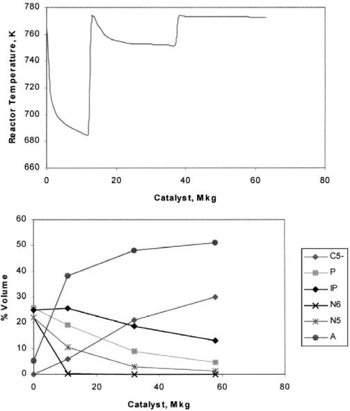
The reforming model results are presented in Figure 8 where the temperature drop and composition profiles of paraffins, naphthenes, and aromatics along the reaction system are shown. Operational conditions and feed naphtha composition used are presented in Table 15. The model reproduces typical unit behavior. Naphthene dehydrogenation results in a sharp temperature drop in the first reactor and the remaining naphthenes disappear along the reactors, increasing the aromatic content and causing minor temperature drops. Hydrocracking reaction produces an increase in C52 hydrocarbons and a

Table 13 Catalytic Reforming Reactions Characteristics

		Equilibrium	Activation
	Heat of reaction	favorable	energy	Rate of
Reaction	(kcal/mol)	conditions	(kcal/mol)	reaction
Isomerization	2–4	T Low	20–25	Medium
Naphthene dehydrogenation	250	High T/low P	20	High
Dehydrocylization	260	High T/low P	35	Low
Hydrocracking	10	Complete	40–50	Low
Coke formation		Complete	30–40	Very Low

578	Larraz and Arvelo

Table 14 Coefficients for the Linear Expression of the

Component j Enthalpy in the i Lump as a Function of

Temperature T. DHj i ¼ mj iT þ bj i

j	mj i	bjI
C6	i ¼ N6, six-carbon-ring naphthenes	2858.7
	0.762
C7	0.772	2900.3
C8	0.783	2912.6
C9	0.793	2924.4
	i ¼ N5, five-carbon-ring naphthenes	2755.1
C6	0.732
C7	0.768	2816.6
C8	0.768	2816.6
C9	0.768	2816.6
	Paraffins
C6	0.793	21082.5
C7	0.794	21052.7
C8	0.792	21015.2
C9	0.792	2984.0
	Aromatics
C6	0.558	305.7
C7	0.585	75
C8	0.606	275.9
C9	0.624	2157.7
	Light hydrocarbons
C1	0.907	22208.6
C2	0.828	21432.8
C3	0.813	21231.0
iC4	0.809	21211.1
nC4	0.801	21145.6
iC5	0.797	21130.5
nC5	0.795	21082.7
	Hydrogen
H2	3.50	2296.8

Source: Ref. 65.

Modeling Catalytic Naphtha Reforming

579

Figure 8 Reaction temperature drop and lumping group composition profiles across reactor system.

decrease in paraffin content of reformate. As the objective is to analyze unit performance with different temperature profiles, an instantaneous simulation is not adequate. More information can be inferred from longer operation times, where coke deposition over the catalyst decreases its activity and higher temperatures are needed to maintain reformate quality. The simulation has been made over a time period of 8000 h similar to a commercial unit run length and using operational conditions analogous to the ones described previously in Table

580		Larraz and Arvelo
Table 15 Operational Parameters and Feed Characteristics for Model use
Parameter	Paraffinic feed	Naphthenic feed
Paraffin	61	40
Naphthene	34	45
Aromatic	5	15
N þ 2A*	44	75
Separator pressure (bar)	22	22
H2/HC ratio	4	4
Initial WAIT (8C)	480	480
Throughput (BPSD)	12000	12000
Loaded catalyst (kg)	11000/21000/26000	11000/21000/26000

*Naphthenes plus twice aromatics.

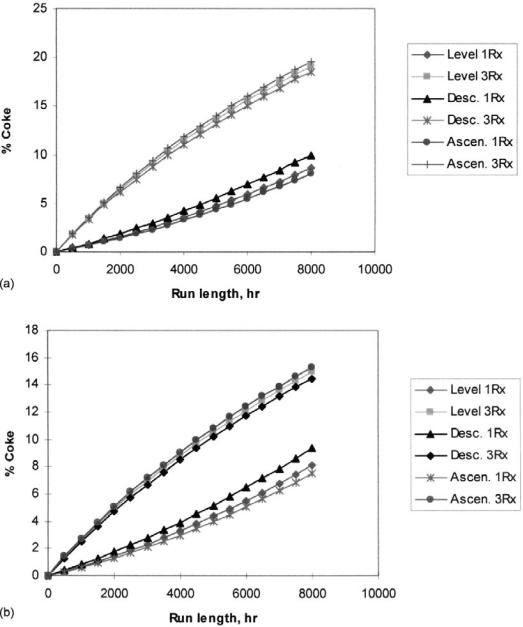
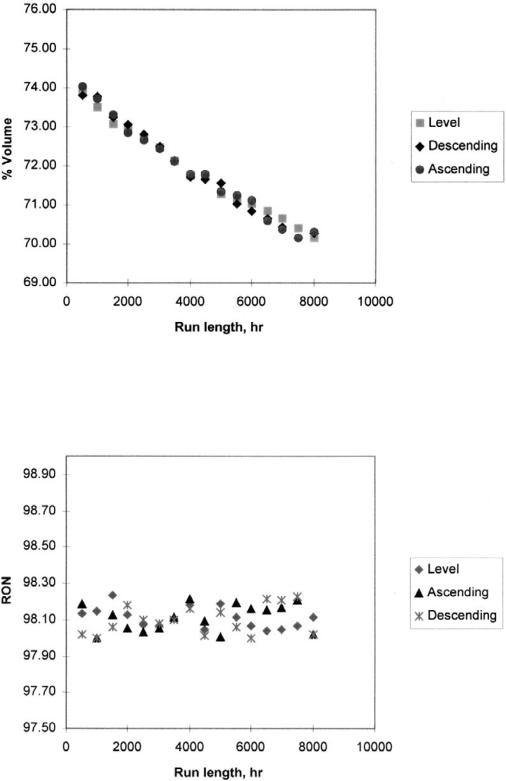
15. The same initial temperature 4808C WAIT was employed. Both high and low Nþ2A feeds are tested to detect first reactor temperature drop influence. Three runs were made employing first a level, then an ascending, and finally a descending profile. A controlling algorithm was implemented that increases inlet reactor temperatures in 18C steps to maintain a 98-RON reformate throughout the run. The reformate octane number is computed as a volumetric average research octane number of the species present in the reformate. Figures 9, 10, and 11 show the reactor carbon content, RON, and reformate yield for each case.

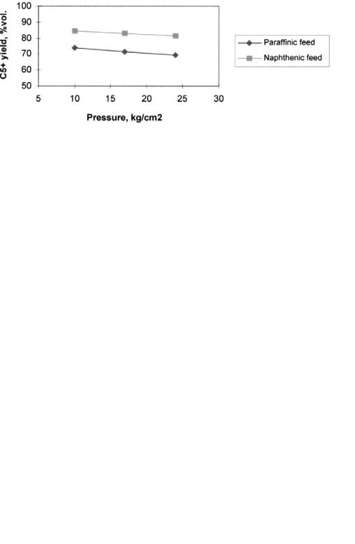
Model results express the higher severity needed in order to increase the RON number for the low naphthene feed. Average-run WABT for the high naphthene feed is 4878C with a final WAIT of 5168C against 4948C and 5238C WAIT for the low-naphthene one. Reformate yield also follows the same behavior. High-naphthene feed reaches an average yield during the course of the run of 81.9% while the low naphthene feed yields 72.2%. Consequently, the reactor carbon content is greater for the paraffinic feed, particularly in the third reactor where the carbon content reaches 19%, as shown in Figure 9.

From the simulation results, some insights regarding reactor temperature profile are obtained. Catalyst deactivation tends to be greatest in the last reactor, and ascending profiles will tend to concentrate coke deposition in this reactor and will reduce the catalyst cycle. For units with furnace temperature limitations at the end of the cycle, starting the cycle with one of the reactors closer to its end of run condition will also limit cycle life.

High-naphthene feeds can cause large temperature drops in the first reactor such that the latter part of the bed in that reactor becomes so cold that the catalyst is quenched and no reaction occurs. Some advantage in this situation may be possible from a descending profile to keep the first reactor bed temperatures higher. A descending profile increases run length due to lower temperature of the

Modeling Catalytic Naphtha Reforming

581

Figure 9 Reactor carbon content. (a) Paraffinic feed. (b) Naphthenic feed.

third reactor and consequently lower degree of cracking reactions. As shown in Figure 9, a 1% decrease in coke content could be obtained. A descending profile produces an increase of around 2% in first reactor coke content due to higher severity. As this reactor presents the lowest coke content, this slight increase could be tolerated so as to permit better use of the loaded catalyst.

With regard to RON and C5þ yield, from the simulation results there does not appear to be significant advantage in shifting temperature profile. As shown in

582	Larraz and Arvelo

Figure 10 C5þ yield for different temperature profiles.

Figure 11 RON for different temperature profiles.

Modeling Catalytic Naphtha Reforming

583

Figures 10 and 11, level profile results in average reactor coke contents, RON, and C5þ yield.

The optimal reactor temperature profile may be established based not only on the reforming unit operation but on other factors due to the paramount role of reforming in the refinery operation. Temperature profile influences reformer performance, and wise use of reactor temperature profiles could extend cycle life if needed although the expected benefits may not compensate operational control and monitoring disadvantages when compared to the level profile operation.

6.3.Benzene Reduction and Reformer Operation Conditions

Refiners are confronted with new specifications for gasoline and these are expected to be followed by more stringent specifications after 2005, although timing and levels are yet to be finalized. Table 16 shows the new specifications that are in the pipeline [66]. One of the most significant changes is the restriction in benzene and aromatics. These proposed regulatory changes directly affect naphtha reforming, as the goal of this process is precisely the production of

Table 16 Evolution of European Gasoline

Specifications

	Property	2000	2005
TVP summer (kPa)		70	60
Sulfur (ppm)		150 max	50 max
Oxygen (wt %)		2.3 max	To be decided
Benzene (vol %)		1.0 max	1.0 max
Aromatics (vol %)		42.0 max	35.0 max
Olefins (vol %)		18.0 max	To be decided
Source: Ref. 66.
Table 17 Trends in Catalytic Reforming Catalysts
	Catalyst changes		Impact
High activity			Higher throughput
High selectivity			More H2 þ aromatics
Low coke formation			Benzene reduction
High thermal stability of the carrier			Higher throughput
			Extended cycle length

Source: Ref. 67.

584	Larraz and Arvelo

Table 18 Benzene Reduction Simulation: Operation Conditions and Feed Compositions, LHSV ¼ 2

	Component	Paraffinic1	Paraffinic2	Naphthenic1	Naphthenic2
P6		11.20	15.00	12.30	8.28
P7		13.40	27.60	15.60	8.79
P8		14.30	18.40	8.87	8.93
P9þ		28.20	5.20	6.80	15.66
CH		1.00	2.60	2.00	4.55
MCP		1.60	3.00	1.71	2.77
N7		4.30	8.80	16.83	14.52
N8		4.80	10.70	11.38	10.78
N9þ		12.10	1.60	9.81	13.95
A6		0.60	0.50	0.90	0.64
A7		1.50	3.70	4.00	3.10
A8		2.90	2.90	6.80	4.25
A9þ	2	4.10	—	3.00	3.78
Pres. (kg/cm )		10	15	25
WAIT paraffinic feed (8C)		499.0	504.5	510.5
WAIT naphthenic feed (8C)		491.2	493.8	501.6
RON		90	94	98

aromatics. Changes in the refinery configuration, including new units such as isomerization, naphtha splitting, and reformate benzene removal, are the first solutions to be implemented [67]. Accomplishing benzene reduction is a potential trend in reforming catalyst design, as shown in Table 17 [67 and references herein].

The benzene content in the reformate is mainly dependent on benzene precursors in the feed and reforming operation conditions [51–53,68,69]. So for a major reduction of benzene content, two basic approaches are possible: either minimize benzene formation by removing benzene precursors from the reformer feed, or fractionate out a light reformate for subsequent conversion or extraction. The use of operating conditions to reduce the benzene formation implies a low-

Table 19 Model Prediction: Aromatic Distribution at

Different Operation Conditions—Paraffinic Feed

Pressure				C8þ (%)
(kg/cm2)	WAIT (8C)	C6 (%)	C7 (%)
20	517	9.8	37.9	51.7
7	506	8.5	34.7	55.4

Modeling Catalytic Naphtha Reforming

585

Figure 12 Influence of pressure on C5þ yield. Model prediction.

severity operation that is frequently beyond the refiners’ capabilities. Despite the low capability of operating variables for benzene reduction, the reforming model previously described has been used to study the effect of temperature and pressure as the main operating variables in the process of benzene formation.

In Table 18, the reformer feed compositions and operation conditions used in the model are shown. Naphthenic as well as paraffinic feeds are treated, with Nþ2A between 45 and 71. The table shows the temperatures needed to obtain the same RON for naphthenic and paraffinic feeds. Operation conditions are typical for a semiregenerative reforming unit. Table 19 shows some results obtained in reforming paraffinic feed. Conversion to aromatics increases as the pressure is reduced. Aromatic distribution shows that the products are mainly toluene and C8 aromatics. There is still not much benzene produced, and results show a slight shift to heavier products at lower pressures. Lower pressures not only increase the conversion to aromatics but also reduce the extent of hydrocracking and hence the loss to light product formation. The general behavior is consistent with the

Figure 13 Influence of reactor temperature on C5þ yield. Model prediction.

586	Larraz and Arvelo

Figure 14 Influence of pressure on C5þ benzene content. Model prediction.

fact that aromatics formation is accompanied by hydrogen production while hydrocracking consumes hydrogen.

An important issue related to operational control of benzene content is reformer C5þ yield. Yield is also a dependent function of feed quality and operating conditions. In Figures 12 and 13, the influence of pressure and temperature on C5þ yields is shown for naphthenic and paraffinic feeds. Temperature is varied from 4908C to 5108C at a constant pressure of 15 kg/cm2. Separator pressure ranges from 10 to 25 kg/cm2 for a constant severity of 98 RON. As expected yield decreases deeply with pressure for the paraffinic feed varying from 73.6 to 69.1 vol %, the naphthenic feed yield loss is lower, i.e., 84.3–81.4 vol %. Yield variation with temperature is much greater than that

Figure 15 Influence of reactor temperature on C5þ benzene content. Model prediction.

Modeling Catalytic Naphtha Reforming

587

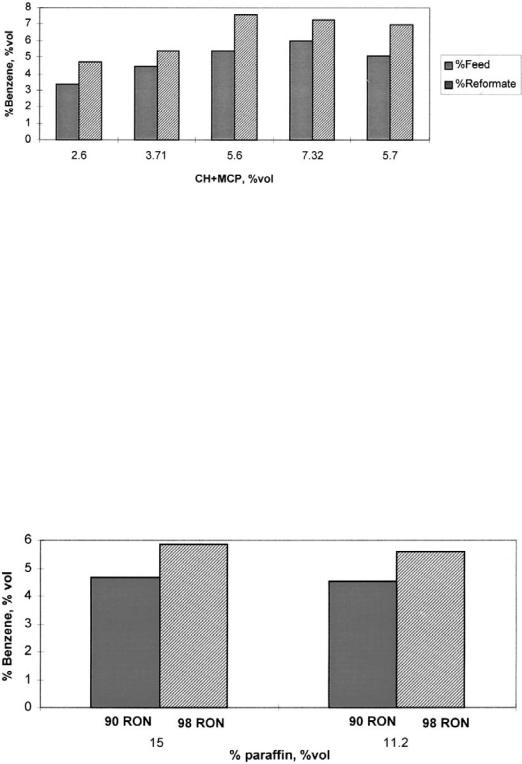
Figure 16 Influence of benzene precursors on C5þ benzene content. Model predictions.

obtained with pressure variations and is again higher for the paraffinic feed, 79.8–71.4 vol %, while naphthenic feed shows a change from 88.5 to 82.9 vol %. The influence of pressure and temperature on reformate benzene content is presented in Figures 14 and 15. The reformate benzene content decreases slightly as the pressure increases; the values obtained are related to the variations in yield and maintain the benzene content almost constant. Naphthenic feed produces higher benzene content, from 5.45 to 5.22 vol %, while the paraffinic feed results in a 1% lower value, from 4.8 to 4.66 vol %. The yield effect previously described becomes less pronounced as temperature increases. Benzene content is higher for naphthenic feeds ranging from 4.2 to 5.3 vol %, while paraffinic feed gives 3.6 to 4.7 vol %. The effect of feed composition for naphthenic feeds gives

Figure 17 Influence of dehydrocyclization on C5þ benzene content. Model predictions.

588	Larraz and Arvelo

reformate with high octane numbers at relatively low temperatures. However, the benzene content of the reformate will in general be higher than in the case of paraffinic feeds.

Benzene precursor influence is shown in Figures 16 and 17, with severity 98 RON and pressure 15 kg/cm2. In Figure 16 the benzene content with respect to reformate and feed is presented against cyclohexane and methylcyclopentane content for different paraffinic and naphthenic feeds. A clear benzene increment is detected as precursors increase. However, the highest benzene content is obtained with a 5.6 vol %, while a higher precursor value, 7.2 vol %, gives lower benzene. The explanation of this apparent contradiction is the paraffin content of each feed. The feed that produces the maximal benzene has 15 vol % of paraffins, with only 11 vol % for the second charge, and due to the high-severity conditions, dehydrocyclization reactions are surely responsible for this high benzene content. To support this argument, in Figure 17 the simulation results for the same feeds but at a lower severity, 90 RON, are presented. As can be seen in the figure, at the lower severity benzene content is reduced overall and the percentage difference for the two feeds is also reduced.

As noted, in the catalytic reforming kinetic model, dehydrocyclization reaction rates are lower than similar dehydrogenation rates and take place in the second and mainly in the third reactor. Also hydrocracking reactions that decrease reformate yield and promote heavy aromatic dealkylation reactions occur in the third reactor, so that one would expect a benzene reduction if thirdreactor severity is decreased. At the same reformate RON, naphthenic feeds need a lower operating temperature, thus diminishing the benzene production due to hydrocracking and dehydrocyclization reactions. Increasing the reformer operating temperature leads to higher dehydrocyclization rates and favors hydrocracking. The reformate yield will be lower and the benzene content of the reformate higher. If one employed pressure reduction, hydrocracking reactions would be suppressed, and octane number as well as yields would be higher, accompanied by a lower benzene content in the reformate. A drawback is that at low pressures more heavy aromatic compounds and coke precursors are formed. Deactivation is therefore much faster at lower pressures.

7CONCLUSION

The applications of the kinetic model for catalytic naphtha reforming to actual refiner issues as exemplified here demonstrate the usefulness of this tool to the refiner. With a model describing the performance of the reforming unit, the refiner can determine at least directionally, if not precisely, the impact of variations in the process conditions or feedstocks available. Additions of other refinery streams as feedstocks can be tested for impact on stability or profltability

Modeling Catalytic Naphtha Reforming

589

without jeopardizing the operation. As will be seen in the chapter on process control, modeling of the reformer is an important aspect in maximizing the utilization of this key refining asset.

ACKNOWLEDGMENTS

The first author thanks Dr. Perez Pascual, head of CEPSA Research Center, for his help during development of this work.

SYMBOLS
Cc	coke content, kg coke/kg cat.
cp	specific heat, kcal/kmolo
dp	particle diameter, cm
De	effective diffusivity, cm2/s
Ei	activation energy of i, cal/mol
Fl,v,t	mixed, liquid, or vapor molar flow rate, kmol/h
G	superficial mass flow rate, kg/m2 h
Hf,l,v	mixed, liquid, or vapor molar enthalpy, kcal/kmol
Ki	vapor liquid distribution coefficient of ith component
ki	rate constant, units consistent with rate expression
k	adiabatic coefficient
Mm	mean molecular weight, kg/kmol
Nc	number of components
Nj	molar flux of j, mol/m2 s
Ojv	vapor fugacity
Pt	total pressure, bar
pi	partial pressure of i, atm
Q	heat balance, kcal/h
ri	reaction rate of ith reaction, kmol/kg cat. h
r0	reaction rate of ith reaction in absence of coke, kmol/kg cat. h
i
Rj	production rate of jth component, kmol/kg cat. h
R	gas constant
T	temperature, 8C
Vj1	liquid fugacity of pure component j
WABT	weight average bed temperature, 8C
WAIT	weight average inlet temperature, 8C
xi	mole fraction of component i in the liquid phase
	calculated parameter
Y
Y	experimental parameter

590	Larraz and Arvelo
yi	mole fraction of component i in vapor phase
z	axial reactor coordinate, m
zj	mole fraction of j in feedstream to the flash drum
g	activity coefficient
rb, f	bulk density of the packing, kg cat./m3; fluid density, kg/m3
rs	catalyst pellet density, kg/m3
V	cross-section of reactor, m2
DHf 0	standard enthalpy of formation, kcal/kmol
1	void fraction of the packing, m3/m3
bji	stoichiometric coefficient of component j in ith reaction
m	viscosity of gas passing through the bed, Pa s
a	deactivation constant, kg cat./kg coke
F	objective function
f	deactivation function

REFERENCES

1.Recasens, E. Combustibles 1955, 78/9, 137–148.

2.Turpin, L.E. Hydrocarbon Processing, June 1992, 81–90.

3.Sowell, R. Hydrocarbon Processing, March 1998, 102–107.

4.Larraz, R. Oil and Gas Eur. Mag. 2000, 2, 33–37.

5.Larraz, R. Honeywell Users Group Conference, Sitges, September 1998.

6.Kugelman, A.M. Hydrocarbon Processing, January 1976, 95–102.

7.Yaws, C.L.; Chiang, P.Y. Hydrocarbon Processing, May 1988, 91–98.

8.Storey, S.H.; Van Zeggeren, F. The Computation of Chemical Equilibria; Cambridge University Press: New York, 1970.

9.White, W.B.; Johnson, S.M.; Dantzig, G.B. J. Chem Phys. 1958, 28, 751.

10.Golfarb, D.; Lapidus, L. I&EC Fundam. February 1968, 7 (1), 141–151.

11.Stull, D.R.; Westrum, E.F.; Sinke, G.C. The Chemical Thermodynamics of Organic Compounds; John Wiley and Sons: New York, 1969.

12.Radosz, M.; Krmarz, J. Hydrocarbon Processing, July 1978, 201–203.

13.Taskar, U.; Riggs, J.H. AICHE J. 1997, 43, (3), 740–753.

14.Brambilla, A.; Trivella, F. Hydrocarbon Processing 1996, 75, (9), 61–66.

15.Twu, C.H.; Coon, J.E. Hydrocarbon Processing 1996 75, (2) 51–56.

16.Riazi, M.R.; Daubert, T.E. Oil and Gas J. August 1986, 50, 25.

17.Lion, A.K.; Edmister, W.C. Hydrocarbon Processing 1975, 54, (8) 119.

18.Riazi, M.R.; Daubert, T.E. Hydrocarbon Processing 1980, 59, (3) 115.

19.Martin, D.L.; Gaddy, J.L. AIChE Symp. Series 1982, 99–107.

20.Luus, R.D. Can. J. Chem. Eng. 1975, 53, 217.

21.Gaines, L.D.; Gaddy, J.L. Ind. Eng. Chem. Proc. Des. Dev. 1976, 15, 206.

22.Jezowski, J.; Poplewski, G.; Madej, S.; Bochenek, R.; Jezowska, A. CHISA Congress, Praga, August 1998.

23.Rossini F.D. et al., API Project 44.

Modeling Catalytic Naphtha Reforming

591

24.Lough, V. Foxboro. Personal communication, 2000.

25.Smith, R.B. Chem. Eng. Prog. 1959, 55, (6) 76.

26.Bommannan, D.; Strivastava, R.D.; Saraf, D.N. Can. J. Chem. Eng. 1989, 67, 405.

27.Barreto, G.F.; Vin˜as, J.M.; Gonzalez, M.G. Lat. Am. Appl. Res. 1996, 26, (1) 21–34.

28.Ansari, R.M.; Tade, M.O. Saudi Aramco J. Technol. Spring 1988, 13–18.

29.Krane, H.G.; Groh, A.B.; Shulman, B.L.; Sinfelt, J.H. World Petroleum Congress, 1960.

30.Aguilar, E.; Anchyeta, J. Oil Gas J. July 25 1994a, 80–83.

31.Aguilar, E.; Anchyeta, J. Oil Gas J. January 31 1994b, 93–95.

32.Burnett, R.L.; Steinmetz, H.L.; Blue, E.M.; Noble, E.M. Petrol Chem. Am. Chem. Soc., Detroit Meeting, April, 1965.

33.Jenkins, J.H.; Stephens, T.W. Hydrocarbon Processing, November 1980, 163–167.

34.Henningsen, J.; Bundgaard-Nielson, M. Br. Chem. Eng. 1970, 15 (11) pp. 1433– 1436.

35.Kmak, W.S. AICHE Meeting, Houston, 1972.

36.Ramage, M.P.; Graziani, K.P.; Krambeck, F.J. Chem. Eng. Sci. 1980, 35, 41–48.

37.Ramage, M.P.; Graziani, K.R.; Shipper, P.H.; Krambeck, F.J.; Choi, B.C. Adv. Chem. Eng. 1987, 13, 193.

38.Lee, J.W.; Ko, K.Y.; Jung, Y.K.; Lee, K.S. Comp. Chem. Eng. 1997, 21, S1105– S1110.

39.Marin, G.B.; Froment, G.F.; Lerou, J.J.; De Backer, W. EFCE 1983, 2 (27), Paris, C117.

40.Marin, G.B.; Froment, G.F. Chem. Eng. Sci. 1982, 37, (5), 759.

41.Van Trimpont, P.A.; Marin, G.B.; Froment, G.F. Ind. Eng. Chem. Res. 1988, 27, 1.

42.Marin, G.B.; Froment, G.F. In The Development and Use of Rate Equations for Catalytic Refinery Process. Proceedings of the 1st Kuwait Conference on Hydrotreating Processes, Kuwait, March 5–9, 1989.

43.Coppens, M.O.; Froment, G.F. Chem. Eng. Sci. 1996, 51, 2283–2292.

44.Galtier, P.; Vacher, P.; Froment, G.F. Hydrocarbon Eng. March 1998, 40–42.

45.Jackson, R. Transport in Porous Catalyst; Elsevier: Amsterdam, 1977.

46.Coppens, M.O.; Froment, G.F. Chem. Eng. Sci. 1995, 50, 1013–1026.

47.Coppens, M.O.; Froment, G.F. Chem. Eng. Sci. 1995, 50, 1027–1039.

48.Coppens, M.O. Catalysis Today 1999, 53, 225–243.

49.Coppens, M.O.; Froment, G.F. Chem. Eng. Sci. 1994, 49, 4897–4907.

50.Weekman, V.W. AICHE J. Monogr. Ser. 1979, 75, 11.

51.Ramage, M.P.; Graziani, K.R.; Shipper, P.H.; Krambeck, F.J.; Choi, B.C. Advances Catalyst 1987, 13, 193.

52.Van Broekhoven, E.H.; Bahlen, F.; Hallie, H. AICHE Spring Meeting, March 1990, 52, 18–20.

53.Pollitzer, E.L.; Hayes, J.C.; Haensel, V. Adv. Chem. Ser. 1970, 97, 20–37.

54.Parera, J.M.; Querini, C.; Figoli, N. Appl. Cat. 1988, 44, L1–L8.

55.Parera, J.M.; Beltramini, J.N. J. Catal. 1988, 112, 357–365.

56.Mieville, R.L. J. Catal. 1986, 100, 482–488.

57.De Pauw, Froment, G.F. Chem. Eng. Sci. 1975, 30, 789–801.

592	Larraz and Arvelo

58.Schro¨der, B.; Salzer, C.; Turek, F. Ind. Eng. Chem. 1991, 30, 326–330.

59.Moore, C.E. Hydrocarbon Processing, July 1991, 92–94.

60.Chao, K.C.; Seader, J.D. AICHE J. 1961, 7, 598.

61.Henley, E.J.; Seader, J.D. Equilibrium Stage Operations in Chemical Engineering; John Wiley and Sons: London, 1981.

62.Pistorius, J.T. Oil Gas J., June 1985, 10, 10–14.

63.Little, D.M. Catalytic Reforming; PennWell: Tulsa, OK, 1983.

64.Levenspiel, O. Chemical Reaction Engineering; Reverte: Barcelona, 1981.

65.Kugelman, A.M. Hydrocarbon Processing, December 1973, 67–70.

66.Genis, O.; Simpson, S.G.; Penner, D.W.; Gautam, R.; Glover, B.K. Hydrocarbon Eng. March 2000, 87–93.

67.Martino, G. 12th International Congress on Catalyst, Stud. Surf. Sci. 2000, 130, 83– 103.

68.Sertic-Bionda, K. Oil Gas Eur. Mag. 1997, 3, 35–37.

69.Ciapetta, F.G. Am. Chem. Soc., Div. Petrol. Chem. 1955, 33, 167.

70.Mandelbrot, B.B. The Fractal Geometry of Nature; Tusquet Eds.: Barcelona, 1997.

71.Pfeifer, P.; Avnir, D. J. Chem. Phys. 1984, 80, 4573.

72.Avnir, D.; Farin, D.; Pfeifer, P. J. Chem. Phys. 1983, 79, 3566–3571.

73.Avnir, D.; Farin, D.; Pfeifer, P. Nature 1984, 308, 261–263.

74.Neimark, A. Physica a 1992, 191, 258–262.

75.Guinier, A.; Fournet, G.; Walker, C.L.; Yudowitch, K.L. Small Angle Scattering of X-Rays; John Wiley and Sons: New York, 1955.

76.Schmidt, P.W. J. Appl. Crystallogr. 1991, 24, 414.

APPENDIX: FRACTALS AND SURFACES

Fractal objects are self-similar structures in which increasing magnifications reveal similar features at different length scales [70]. They show a power-law relation between a certain properties (like mass, void volume, or surface area) and length scale. These are termed mass fractal, pore fractal, and surface fractal, respectively [71]. Characterization and analysis of porous objects in terms of fractal geometry has become an intensive research area in recent years. Experiments show a large number of natural and industrial structures having either fractal surfaces or fractal pore distribution [72]. Fractals have been described as objects capable of simulating diffusion-controlled process structures as catalysts [73]. Their use enables important observations to be made when analyzing much of the adsorption data published so far for a large number of porous media, including many catalysts. The measured surface area S depends on the effective diameter d of the sorbate molecules according to simple power law:

S d a

ðA1Þ

More precisely, when data are plotted as log S vs. log d, a straight line can be fitted, with a slope between 0 and 1. If a ¼ 0, the surface area does not depend on

Modeling Catalytic Naphtha Reforming

593

the size of the probe. Frequently a is found to be greater than 0, implying that specific area is meaningless without specifying the resolution d. The so-called fractal dimension, D, expresses the space filling capacity of a fractal, while Euclidean shapes have integer dimensions (1 for a line, 2 for a surface, and 3 for a volume), a catalyst surface can have any dimension between 2 and 3, both limits included. Many fractals in nature can be very well approximated by a statistical self-similar or self-affine structure. A real object can only be a self-similar fractal, within a finite fractal scaling range, denoted with the inner and outer cutoffs, dmin and dmax. Informally the number N of units of size d needed to cover a fractal object decreases with d as:

N d D

ðA2Þ

Lengths are measured as Nd, areas as Nd2, so that in equation (A1), a ¼ 12D and becomes

S d2 D

ðA3Þ

Methods for fractal dimension determination have been described using the information of the complete adsorption isotherm of a single probe [74]. Smallangle X-ray scattering can be also used to study the mass fractal and surface morphology of materials [75,76].