Varian Microeconomics Workout

Consumption

400

300

200

100

0	20	40	60	80
				Leisure

9.10 (0) In the United States, real wage rates in manufacturing have risen steadily from 1890 to the present. In the period from 1890 to 1930, the length of the workweek was reduced dramatically. But after 1930, despite the continuing growth of real wage rates, the length of the work week has stayed remarkably constant at about 40 hours per week.

Hourly Wages and Length of Work Week

in U.S. Manufacturing, 1890{1983

Sources: Handbook of Labor Statistics, 1983 and U.S. Economic History, by Albert Niemi (p. 274). Wages are in 1983 dollars.

Year	Wage	Hours Worked
1890	1.89	59.0
1909	2.63	51.0
1920	3.11	47.4
1930	3.69	42.1
1940	5.27	38.1
1950	6.86	40.5
1960	8.56	39.7
1970	9.66	39.8
1983	10.74	40.1

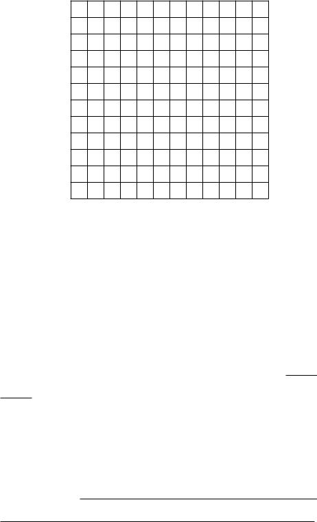
(a) Use these data to plot a \labor supply curve" on the graph below.

Hourly wage rate (in 1983 dollars)

12

10

8

6

4

2

0	10	20	30	40	50	60
			Hours of work per week

(b) At wage rates below $4 an hour, does the workweek get longer or

shorter as the wage rate rises?

.

(c) The data in this table could be consistent with workers choosing various hours a week to work, given the wage rate. An increase in wages has both an endowment income e®ect and a substitution e®ect.

The substitution e®ect alone would make for a (longer, shorter)

workweek. If leisure is a normal good, the endowment income

e®ect tends to make people choose (more, less)					leisure and
a (longer, shorter)		workweek. At wage rates below $4 an
hour, the (substitution, endowment income)						e®ect

appears to dominate. How would you explain what happens at wages above $4 an hour?

.

(d) Between 1890 and 1909, wage rates rose by								percent, but
weekly earnings rose by only			percent. For this period, the gain
in earnings (overstates, understates)						the gain in workers'
wealth, since they chose to take (more, less)							leisure in 1909
than they took in 1890.

9.11 (0) Professor Mohamed El Hodiri of the University of Kansas, in a classic tongue-in-cheek article \The Economics of Sleeping," Manifold, 17 (1975), o®ered the following analysis. \Assume there are 24 hours in a day. Daily consumption being x and hours of sleep s, the consumer maximizes a utility function of the form u = x2s, where x = w(24 ¡ s), with w being the wage rate."

(a) In El Hodiri's model, does the optimal amount of sleeping increase,

decrease, or stay the same as wages increase?

.

(b) How many hours of sleep per day is best in El Hodiri's model?

.

9.12 (0) Wendy and Mac work in fast food restaurants. Wendy gets $4 an hour for the ¯rst 40 hours that she works and $6 an hour for every hour beyond 40 hours a week. Mac gets $5 an hour no matter how many hours he works. Each has 80 hours a week to allocate between work and leisure and neither has any income from sources other than labor. Each has a utility function U = cr, where c is consumption and r is leisure. Each can choose the number of hours to work.

(a) How many hours will Mac choose to work?		.

(b) Wendy's budget \line" has a kink in it at the point where r =

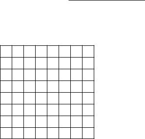
and c = Use blue ink for the part of her budget line where she would be if she does not work overtime. Use red ink for the part where she would be if she worked overtime.

Consumption

400

300

200

100

0	20	40	60	80
				Leisure

(c) The blue line segment that you drew lies on a line with equation

The red line that you drew lies on a line with equation

(Hint: For the red line, you know one point on the line and you know its slope.)

(d) If Wendy was paid $4 an hour no matter how many hours she worked,

she would work hours and earn a total of a week. On your graph, use black ink to draw her indi®erence curve through this point.

(e) Will Wendy choose to work overtime?				What is the best
choice for Wendy from the red budget line? (c; r) =					How
many hours a week will she work?						.

(f) Suppose that the jobs are equally agreeable in all other respects. Since Wendy and Mac have the same preferences, they will be able to agree

about who has the better job. Who has the better job? (Hint: Calculate Wendy's utility when she makes her best choice. Calculate what her utility would be if she had Mac's job and chose the best amount of time to work.)

9.13 (1) Wally Piper is a plumber. He charges $10 per hour for his work and he can work as many hours as he likes. Wally has no source of income other than his labor. He has 168 hours per week to allocate between labor

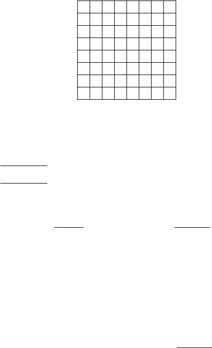
and leisure. On the graph below, draw Wally's budget set, showing the various combinations of weekly leisure and income that Wally can a®ord.

Income

2400

2000

1600

1200

800

400

0	40	80	120	160	200	240
						Leisure

(a) Write down Wally's budget equation.

.

(b)While self-employed, Wally chose to work 40 hours per week. The construction ¯rm, Glitz and Drywall, had a rush job to complete. They o®ered Wally $20 an hour and said that he could work as many hours as he liked. Wally still chose to work only 40 hours per week. On the graph you drew above, draw in Wally's new budget line.

(c)Wally has convex preferences and no kinks in his indi®erence curves. On the graph, draw indi®erence curves that are consistent with his choice of working hours when he was self-employed and when he worked for Glitz and Drywall.

(d)Glitz and Drywall were in a great hurry to complete their project and wanted Wally to work more than 40 hours. They decided that instead of paying him $20 per hour, they would pay him only $10 an hour for the ¯rst 40 hours that he worked per week and $20 an hour for every hour of \overtime" that he worked beyond 40 hours per week. On the graph that you drew above, use red ink to sketch in Wally's budget line with this pay schedule. Draw the indi®erence curve through the point that Wally chooses with this pay schedule. Will Wally work more than 40 hours or

less than 40 hours per week with this pay schedule?

.

9.14 (1) Felicity loves her job. She is paid $10 an hour and can work as many hours a day as she wishes. She chooses to work only 5 hours a day. She says the job is so interesting that she is happier working at this job than she would be if she made the same income without working at all. A skeptic asks, \If you like the job better than not working at all, why don't you work more hours and earn more money?" Felicity, who is entirely rational, patiently explains that work may be desirable on average but undesirable on the margin. The skeptic insists that she show him her indi®erence curves and her budget line.

(a) On the axes below, draw a budget line and indi®erence curves that are consistent with Felicity's behavior and her remarks. Put leisure on the horizontal axis and income on the vertical axis. (Hint: Where does the indi®erence curve through her actual choice hit the vertical line l = 24?)

9.15 (2) Dudley's utility function is U(C; R) = C ¡ (12 ¡ R)2, where R is the amount of leisure he has per day. He has 16 hours a day to divide between work and leisure. He has an income of $20 a day from nonlabor sources. The price of consumption goods is $1 per unit.

(a) If Dudley can work as many hours a day as he likes but gets zero

wages for his labor, how many hours of leisure will he choose?

.

(b) If Dudley can work as many hours a day as he wishes for a wage

rate of $10 an hour, how many hours of leisure will he choose?

How many hours will he work? (Hint: Write down Dudley's budget constraint. Solve for the amount of leisure that maximizes his utility subject to this constraint. Remember that the amount of labor he wishes to supply is 16 minus his demand for leisure.)

(c) If Dudley's nonlabor income decreased to $5 a day, while his wage rate

remained at $10, how many hours would he choose to work? .

(d) Suppose that Dudley has to pay an income tax of 20 percent on all of his income, and suppose that his before-tax wage remained at $10 an hour and his before-tax nonlabor income was $20 per day. How many

hours would he choose to work?

.

(1+r)

m2

The theory of consumer saving uses techniques that you have already learned. In order to focus attention on consumption over time, we will usually consider examples where there is only one consumer good, but this good can be consumed in either of two time periods. We will be using two \tricks." One trick is to treat consumption in period 1 and consumption in period 2 as two distinct commodities. If you make period-1 consumption the numeraire, then the \price" of period-2 consumption is the amount of period-1 consumption that you have to give up to get an extra unit of period-2 consumption. This price turns out to be 1=(1 + r), where r is the interest rate.

The second trick is in the way you treat income in the two di®erent periods. Suppose that a consumer has an income of m1 in period 1 and m2 in period 2 and that there is no in°ation. The total amount of period- 1 consumption that this consumer could buy, if he borrowed as much money as he could possibly repay in period 2, is m1 + 1+m2r . As you work the exercises and study the text, it should become clear that the consumer's budget equation for choosing consumption in the two periods is always

c1 + 1 c+2 r = m1 + 1m+2r :

This budget constraint looks just like the standard budget constraint that you studied in previous chapters, where the price of \good 1" is 1, the price of \good 2" is 1=(1 + r), and \income" is m1 + . Therefore if you are given a consumer's utility function, the interest rate, and the consumer's income in each period, you can ¯nd his demand for consumption in periods 1 and 2 using the methods you already know. Having solved for consumption in each period, you can also ¯nd saving, since the consumer's saving is just the di®erence between his period-1 income and his period-1 consumption.

A consumer has the utility function U(c1; c2) = c1c2. There is no in°ation, the interest rate is 10%, and the consumer has income 100 in period 1 and 121 in period 2. Then the consumer's budget constraint c1 +c2=1:1 = 100 + 121=1:1 = 210: The ratio of the price of good 1 to the price of good 2 is 1 + r = 1:1. The consumer will choose a consumption bundle so that MU1=MU2 = 1:1. But MU1 = c2 and MU2 = c1, so the consumer must choose a bundle such that c2=c1 = 1:1. Take this equation together with the budget equation to solve for c1 and c2. The solution is c1 = 105 and c2 = 115:50. Since the consumer's period-1 income is only 100, he must borrow 5 in order to consume 105 in period 1. To pay back principal and interest in period 2, he must pay 5.50 out of his period-2 income of 121. This leaves him with 115.50 to consume.

You will also be asked to determine the e®ects of in°ation on consumer behavior. The key to understanding the e®ects of in°ation is to see what happens to the budget constraint.

Suppose that in the previous example, there happened to be an in°ation rate of 6%, and suppose that the price of period-1 goods is 1. Then if you save $1 in period 1 and get it back with 10% interest, you will get back $1.10 in period 2. But because of the in°ation, goods in period 2 cost 1.06 dollars per unit. Therefore the amount of period-1 consumption that you have to give up to get a unit of period-2 consumption is 1:06=1:10 = :964 units of period-2 consumption. If the consumer's money income in each period is unchanged, then his budget equation is c1 + :964c2 = 210. This budget constraint is the same as the budget constraint would be if there were no in°ation and the interest rate were r, where :964 = 1=(1 + r). The value of r that solves this equation is known as the real rate of interest. In this case the real rate of interest is about :038. When the interest rate and in°ation rate are both small, the real rate of interest is closely approximated by the di®erence between the nominal interest rate, (10% in this case) and the in°ation rate (6% in this case), that is, :038 » :10 ¡ :06. As you will see, this is not such a good approximation if in°ation rates and interest rates are large.

10.1 (0) Peregrine Pickle consumes (c1; c2) and earns (m1; m2) in periods 1 and 2 respectively. Suppose the interest rate is r.

(a) Write down Peregrine's intertemporal budget constraint in present

value terms.

.

(b) If Peregrine does not consume anything in period 1, what is the most

he can consume in period 2?			This is the (future value,
present value) of his endowment.				.

(c) If Peregrine does not consume anything in period 2, what is the most

he can consume in period 1?				This is the (future value,
present value) of his endowment.					What is the slope
of Peregrine's budget line?						.

10.2 (0) Molly has a Cobb-Douglas utility function U(c1; c2) = ca1c12¡a, where 0 < a < 1 and where c1 and c2 are her consumptions in periods 1 and 2 respectively. We saw earlier that if utility has the form u(x1; x2) = xa1x12¡a and the budget constraint is of the \standard" form p1x1 +p2x2 = m, then the demand functions for the goods are x1 = am=p1 and x2 = (1 ¡ a)m=p2.