6 Model file format

39

6.3.2 AddExplicitVar

Heading

function AddExplicitVar(var Variable : TFloat; Name : PChar; DoPlot : TBoolean) : TInteger;

function AddExplicitVarExt(var Variable : TFloat; Name : PChar; DoPlot : TBoolean; ALabel : PChar) : TInteger;

Parameters
Variable	The declared pascal variable, which represents the explicit variable
Name	in the model.
	Name of explicit variable.
DoPlot	True:	The variable is plotted.
Example	False:	The variable is added to the Results page when calculation is done.

AddExplicitVar(W,'Compressor work', True);

6.3.3 SetSampleTime

Heading

procedure SetSampleTime(IsFixed : Boolean; Value : TFloat);

Parameters

IsFixed Run with fixed sample time? If true the sample time specified in value is used;

else fixed sample time is not used.

Value The value of the fixed sample time in seconds.

Example

SetSampleTime(True,10);

6.4 ModelEquations

In the ModelEquations procedure the equations are written. ModelEquations is called every time the Solver needs to evaluate the model.

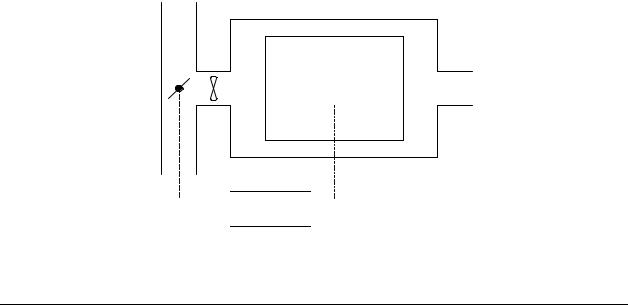
Suppose the problem from chapter 5 is extended, so that instead of just cooling the block, it is required that the temperature is held at 50 °C ± 2 °C. To accomplish this, the block is put into an air chamber, with the possibility to add air at 70°C or air at 20°C:

Th

ρ,V,cp ,T

T c Controller

Figure 10. Controlling the temperature.

WinDali

Morten Juel Skovrup

40 6 Model file format

Now the system has two states: either hot air supply or cold air supply. The equations for the two states are:

ρVcp ddTt = h A(Tc −T ) ,Cold

(5.1)

ρVcp ddTt = h A(Th −T ) , Hot

The SetupProblem procedure for this case will look like this:

procedure SetupProblem; begin

SetupModel('Cooling of block 2',0,20000); SetStates('Cold,Hot'); SetParamPages('Material,Geometry,"Heat transfer"'); AddDynamic(T,100,'T','Temperature [°C]'); AddFloatParamExt(Rho,8000,'Density [kg/m^3]',1,0,20000,'');

AddFloatParamExt(Cp0,480,'Specific heat [J/kg K]',1,0.001,5000,''); AddFloatParamExt(Lambda,15,'Conductivity [W/m K]',1,0.0001,5000,''); AddFloatParamExt(V,0.001,'Volume [m^3]',2,0.000001,1000,''); AddFloatParamExt(A,0.06,'Surface area [m^2]',2,0.000001,10000,''); AddFloatParamExt(h,10,'Heat transfer coefficient [W/m^2 K]',

3,0.00001,100000,'');

AddFloatParamExt(Tc,20,'Cold temperature [°C]',3,0,0,''); AddFloatParamExt(Th,70,'Hot temperature [°C]',3,0,0,''); AddExplicit(Bi,'Biot number',False);

end;

and the ModelEquations procedure will look like this:

procedure ModelEquations(Time : TFloat; State : TInteger; var R : array of TFloat; var YDot : array of TFloat);

begin

if State = 1 then

YDot[0] := h*A/(Rho*V*Cp)*(Tc-T) else

YDot[0] := h*A/(Rho*V*Cp)*(Th-T); end;

It is also necessary to fill out StateShift but this will be treated in chapter 6.5.

To show how static equations are formulated assume that the specific heat of the material, no longer is constant; but can be calculated as:

	cp = cp0	cp −T	(5.2)
		cp

Note that this equation is pure fictional. It has no physical meaning and only serves to illustrate static variables. cp0 is a parameter provided by the user.

WinDali

Morten Juel Skovrup

6 Model file format

41

In SetupProblem the following line:

AddFloatParamExt(Cp,480,'Specific heat [J/kg K]',1,0.001,5000,'');

Is changed to:

AddFloatParamExt(Cp0,480,'Specific heat [J/kg K]',1, 0.001,5000,'');

And the following line is added to SetupProblem:

AddCommonStaticExt(Cp,480,'Cp','Specific heat [J/kg K]','',0,0,True,'');

The cp equation also has to be added to ModelEquations. This is done by adding the line:

R[0] := Cp-Cp0*Sqrt((Cp-T)/Cp);

See also the included "Cooling of Block 2" demo.

6.5 StateShift

StateShift is used to specify when the logical state is changed. The heading of the StateShift function looks like this:

procedure StateShift(Time : TFloat; State : TInteger; var G : array of TFloat);

The G-array is zero-indexed, and has the same length as the number of states. A shift to another state is done when the corresponding item in the G array becomes negative. The State parameter holds the number of the current state.

In the example from chapter 6.4 there was two states:

1:Cold corresponds to G[0]

2:Hot corresponds to G[1]

The temperature should be held at 50 °C ± 2 °C. That is when the system is in state 1 it should shift to state 2 when the temperature drops below 48 °C. And when the system is in state 2 it should shift to state 1 when the temperature is above 52 °C:

procedure StateShift(Time : TFloat; State : TInteger; var G : array of TFloat);

begin

case State of

1 : G[1] := T-48;

2 : G[0] := 52-T; end;

end;

What the code states is that when the current state is 1 (Cold) then G[1] becomes negative when T is less than 48 °C and the Solver will then shift to state 2. When the current state is 2 (Hot) then G[0] will become negative when T is larger than 52 °C, and the Solver will then shift to state 1.

WinDali

Morten Juel Skovrup

42 6 Model file format

The procedure ShiftToState can be used to perform the same as the code above, but it makes it a bit more readable:

procedure StateShift(Time : TFloat; State : TInteger; var G : array of TFloat);

begin

case State of

1 : SwitchToState(2,T-48,G);

2 : SwitchToState(1,52-T,G); end;

end;

Read the call SwitchToState(2,T-48,G) as "Switch to state 2 when T-48 becomes negative".

Remember to supply G as the last parameter in the call to SwitchToState.

SwitchToState has the following implementation:

procedure SwitchToState(StateNum : TInteger; SignChange : TFloat; var G : array of TFloat);

begin

G[StateNum-1] := SignChange; end;

6.6 OnStateChange

OnStateChange is seldom modified. It can be used to supply guesses (different from the default) on the static variables or to change the “initial” value of a dynamic variable before continuing in to a new state. An example showing this is included in the Bouncing Ball demo

The solver supplied with WinDali automatically updates guesses on static variables. That is it uses the supplied guesses the first time it enters a state. If it enters the same state a second time, the solution from the first time is used as guesses.

6.7 OnSolution

Called every time a solution has been found. Can be used to do intermediate calculations.

6.8 OnSample

The procedure OnSample is called if you choose to run the simulation with a fixed sample time.

If for example the sample time is 10 seconds it forces the equation solver to produce a solution at every 10 seconds, but it might also produce solutions in between each sample.

When a solution is found at a sample time, then first OnSolution is called then OnSample and finally OnSolution again. The reason for this is that you want to plot both the solution just before OnSample is called, and if some values are changed in OnSample, then the changes should also be plotted with the same timestamp.

If you for example implement a controller, which operates with a fixed sample time of 10 seconds – let us say it controls the speed of a compressor – then at time 100 a solution is found

WinDali

Morten Juel Skovrup

6 Model file format

43

which is plotted. This solution is then used in the controller when OnSample is called to change the speed, and finally OnSolution is called to reflect the change in the speed.

You should note that OnSample will not be called at the initial time. If your simulation runs from 0 secods and you specify a sample time of 10 secondes then OnSample will be called the first time at Time = 10 seconds. This is because the results of the calculations in OnSample might be used in ModelEquations and the static and dynamic variables might be used in OnSample. At the initial time the static variables only have guess-values, so to solve the equations in ModelEquations the results from OnSample has to be known. In other words: you have to specify initial values for the values calculated in OnSample, which are used in ModelEquations.

Typically a controller will also control which state the system is in (for example if the compressor is On or Off). Therefore you can force the state to change by changing the supplied State parameter in OnSample:

procedure OnSample(Time : TFloat; var State : TInteger);

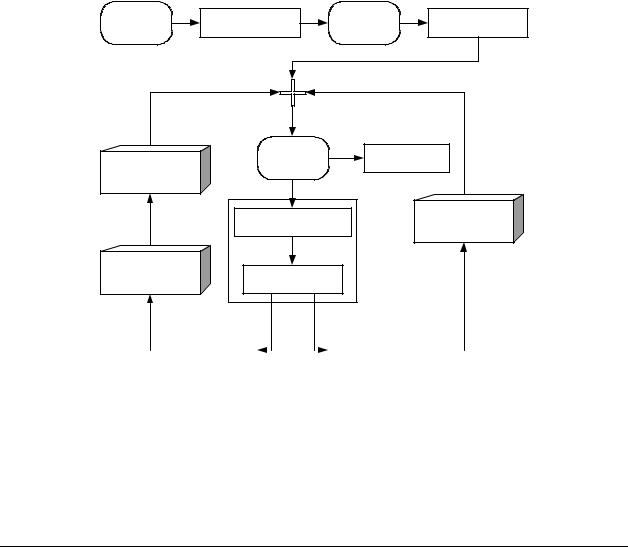
Note that State is a var parameter, which means that you can change State within OnSample. The calling sequence for the procedures in figure 8 was:

	1) Load	2)	SetUpProblem	3) Start	4) PreCalc
	Model

	State Change	5) Stop	Yes	10) EndCalc
	Procedure
		No
	6)	ModelEquations		Sample Check
				Procedure
	Sample Check	7) StateShift
	Procedure
	Yes		No

	8) OnSolution						9) OnSolution

Figure 8. Calling sequence for the procedures in the model file.

And the State Change Procedure called the following procedures:

WinDali

Morten Juel Skovrup