5 Creating a simple model

15

First you have to define the variables and parameters so Free Pascal knows about them. This is done by writing the following right after implementation:

implementation const

Rho	= 8000;
Cp	= 480;
Lambda	= 15;
V	= 0.001;
A	= 0.06;
h	= 10;
Ta	= 20;
var

T : TFloat;

Bi : TFloat;

5.1 SetupProblem

In the procedure SetupProblem you have to tell the system about the variables, parameters and states in your problem. This also specifies the user-interface of the Simulation Interface program.

You tell the system about your problem by calling a number of predefined functions. The ones you need to know about for this simple problem will be shortly explained (details are given in chapter 6).

SetupModel(Title : PChar; TStart,TEnd : TFloat);

This function specifies the title of your problem and the time you want to simulate. For this simple problem, let us say that you want to simulate 1000 seconds so you should call

SetupModel like this:

SetupModel('Simple problem',0,1000);

AddDynamic(var Variable : TFloat; InitalValue : TFloat; Name,LongName : PChar);

This function is used to specify detailed information about each of the dynamic variables in the problem. The individual parameters are explained in detail in chapter 6. There is only one dynamic variable and lets say the initial value is 100 °C:

AddDynamic(T,100,'T','Temperature [°C]');

AddExplicit(var Variable : TFloat; Name : PChar; DoPlot : TBoolean);

Add variables you can calculate explicitly, but want to display the value of:

AddExplicit(Bi,'Biot number',False);

This completes the SetupProblem procedure.

WinDali

Morten Juel Skovrup

16 5 Creating a simple model

5.2 ModelEquations

In ModelEquations you specify the equations. The heading looks like this:

procedure ModelEquations(Time : TFloat; State : TInteger; var R : array of TFloat; var YDot : array of TFloat);

This procedure is called every time the solver needs to do calculations on your model. The parameters in the procedure heading are:

•Time The current simulation time (in seconds)

•State The current state (as there is only one state in this example, this will always be

equal to 1)

•R A zero-based vector where you should return a residual for each of the static

equations in your model. As there are no static equations in this model, R can be ignored.

•YDot A zero-based vector where you should return the derivatives of the dynamic

variables in your model.

A zero-based vector means that the first place in the vector is indexed 0, the second place 1 and so on. For the simple model there is only 1 dynamic variable and no static variables. Note that because of the registration of the dynamic variable (calling AddDynamic), the Pascal variable T will always have the correct and updated values when ModelEquations is called.

If equation (4.2) is arranged so the derivative is isolated, the programming ModelEquations of is straightforward:

d T	=	h A	(Ta −T )	(4.3)
d t
		ρV cp

procedure ModelEquations(Time : TFloat; State : TInteger; var R : array of TFloat; var YDot : array of TFloat);

begin

YDot[0] := h*A/(Rho*V*Cp)*(Ta-T); end;

This concludes the ModelEquations procedure.

5.3 EndCalc

EndCalc is called once at the end of the simulation. The only thing left to be calculated is the Biot number:

procedure EndCalc(Time : TFloat; State : TInteger); begin

Bi := h*V/(A*Lambda); end;

WinDali

Morten Juel Skovrup

5 Creating a simple model

17

In full the file ModelMain.pp looks like this:

unit ModelMain;

interface

uses mjsDLLTypes,UmjsKernelTypes;

{$I ModelInterface.inc} implementation

const

Rho = 8000; Cp = 480; Lambda = 15; V = 0.001; A = 0.06; h = 10; Ta = 20; var

T,Bi : TFloat;

procedure SetupProblem; begin

SetupModel('Simple problem',0,1000); AddDynamic(T,100,'T','Temperature [°C]'); AddExplicit(Bi,'Biot number',False);

end;

procedure PreCalc(Time : TFloat; State : TInteger); begin

end;

procedure ModelEquations(Time : TFloat; State : TInteger; var R : array of TFloat; var YDot : array of TFloat);

begin

YDot[0] := h*A/(Rho*V*Cp)*(Ta-T); end;

procedure StateShift(Time : TFloat; State : TInteger; var G : array of TFloat);

begin end;

procedure OnStateChange(Time : TFloat; OldState,NewState : TInteger); begin

end;

procedure OnSolution(Time : TFloat; State : TInteger); begin

end;

procedure OnSample(Time : TFloat; var State : TInteger); begin

end;

procedure EndCalc(Time : TFloat; State : TInteger); begin

Bi := h*V/(A*Lambda); end;

procedure OnQuit; begin

end;

procedure OnUIValueChange(UIType : TInteger; Num,State,Choice : TInteger; Value : TFloat);

begin end;

procedure OnSaveSettings(FileName : PChar); begin end; procedure OnLoadSettings(FileName : PChar); begin end; end.

WinDali

Morten Juel Skovrup

18 5 Creating a simple model

5.4 Compiling

Now it is time to compile the model. Select the Model|Compile menu and note if there is any error messages in the Message window. If you have made an error you can double-click it in the Message window and the error will be highlighted in your code. If no errors occurred you can run a simulation by selecting the Simulate|Run menu. The resulting model file will have the extension “.mdl”.

5.5 Simulation

When you select the Simulate|Run menu in the Model Editor you start the simulation program. If the model file was created exactly as described above, you will see the following screen:

Figure 6. The Simulation Interface program

In the General page the simulation time can be set by the user (i.e. the values specified in the call to SolverSettings was only default values).

The rest of the values in the General, Cases and Solver pages will be explained in chapter 10.

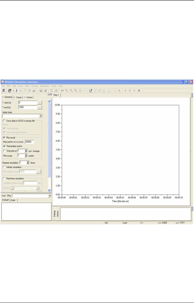
To start the simulation, select the Simulation|Start menu or press the <Play> button on the toolbar. In either case the result should look like this:

WinDali

Morten Juel Skovrup

5 Creating a simple model

19

Figure 7. Simulation result.

This shows that the simulation time was to short. Try increasing the simulation end-time to for example 1 day (86400 seconds), and run the simulation again.

If you want to change for example the density Rho to 1000, then you have to go back to the Model Editor, change Rho and recompile the model. Instead you could install Rho as a parameter in the model (together with the rest of the constants you defined in the model). This is done by changing the model to the following:

WinDali

Morten Juel Skovrup

20 5 Creating a simple model

implementation var

T,Bi : TFloat; Rho,Cp,Lambda,V,A,h,Ta : TFloat;

procedure SetupProblem; begin

SetupModel('Simple problem',0,1000); SetParamPages('Parameters'); AddDynamic(T,100,'T','Temperature [°C]'); AddExplicit(Bi,'Biot number',False); AddFloatParam(Rho,8000,'Density [kg/m^3]',1); AddFloatParam(Cp,480,'Specific heat [J/kg K]',1); AddFloatParam(Lambda,15,'Conductivity [W/m K]',1); AddFloatParam(V,0.001,'Volume [m^3]',1); AddFloatParam(A,0.06,'Surface area [m^2]',1); AddFloatParam(h,10,'Heat transfer coefficient [W/m^2 K]',1); AddFloatParam(Ta,20,'Ambient temperature [°C]',1);

end;

Note that now Rho,Cp etc. are defined as Pascal variables instead of constants, and that a call to

SetParamPages has been added.

When you compile the model and run it, you will see the following page in the Simulation Interface program:

Now you can change the parameters in the Simulation Interface program, without having to recompile the model.

WinDali

Morten Juel Skovrup