Radiation Physics for Medical Physiscists - E.B. Podgorsak

2.4 Multi-electron Atoms

69

•According to Pauli’s exclusion principle in a multi-electron atom no two electrons can have all four quantum numbers identical.

•The energy and position of each electron in a multi-electron atom are most a ected by the principal quantum number n. The electrons that have the same value of n in an atom form a shell.

•Within a shell, the energy and position of each electron are a ected by the value of the orbital angular momentum quantum number . Electrons that have the same value of in a shell form a sub-shell.

•The specification of quantum numbers n and for each electron in a multi-electron atom is referred to as the electronic configuration of the atom.

•Pauli’s exclusion principle confirms the shell structure of the atom as well as the sub-shell structure of individual atomic shells:

– Number of electrons in sub-shells that are labeled with quantum num-

bers n, , m :

2(2 + 1)

	–	Number of electrons in sub-shells that are labeled with quantum num-
		bers n, , j:		(2j + 1)
	–	Number of electrons in a shell:		(2 + 1) = 2n2
			2 n−1
			=0

The main characteristics of atomic shells and sub-shells are given in Tables 2.2 and 2.3, respectively. The spectroscopic notation for electrons in the K, L, and M shells and associated sub-shells is given in Table 2.4.

Table 2.2. Main characteristics of atomic shells

Principal quantum number n	1	2	3	4	5
Spectroscopic notation	K	L	M	N	O
Maximum number of electrons	2	8	18	32	–
Table 2.3. Main characteristics of atomic subshells
Orbital quantum number	0	1	2	3
Spectroscopic notation	s	p	d	f
Maximum number of electrons	2	6	10	14

Table 2.4. Notation for electrons in the K, L, M shells of a multi-electron atom

Principal quantum number n

Orbital angular momentum and total angular momentum j of electron

s1/2 p1/2 p3/2 d3/2 d5/2 f

1	K
2	LI	LII	LIII
3	MI	MII	MIII	MIV	MV

70 2 Rutherford–Bohr Atomic Model

2.4.2 Hartree’s Approximation for Multi-electron Atoms

Bohr’s theory works well for one-electron structures (hydrogen atom, singly ionized helium, doubly ionized lithium, etc.) but does not apply directly to multi-electron atoms because of the repulsive Coulomb interactions among electrons constituting the atom. These interactions disrupt the attractive Coulomb interaction between an orbital electron and the nucleus and make it impossible to predict accurately the potential that influences the kinematics of the orbital electron. Douglas Hartree proposed an approximation that predicts the energy levels and radii of multi-electron atoms reasonably well despite its inherent simplicity.

Hartree assumed that the potential seen by a given atomic electron is given by

V (r) = −	Ze e2 1	,	(2.79)
	4πεo r

where

Ze is the e ective atomic number,

Ze e is an e ective charge that accounts for the nuclear charge Ze as well as for the e ects of all other atomic electrons.

Hartree’s calculations show that in multi-electron atoms the e ective atomic number Ze for K-shell electrons (n = 1) has a value of about Z − 2. Charge distributions of all other atomic electrons produce a charge of about −2e inside a sphere with the radius of the K shell, partially shielding the K- shell electron from the nuclear charge +Ze and producing an e ective charge Ze e = (Z − 2)e.

For outer shell electrons Hartree’s calculations show that the e ective atomic number Ze approximately equals n, where n specifies the principal quantum number of the outermost filled shell of the atom in the ground state.

Based on Bohr’s one-electron atom model, Hartree’s relationships for the radii rn of atomic orbits (shells) and the energy levels En of atomic orbits are given as follows:

rn =	aon2						(2.80)
	Ze
and
En = −ER			n			2	(2.81)
						.
				Ze

Hartree’s approximation for the K-shell (n = 1) electrons in multi-electron atoms then results in the following expressions for the K-shell radius and K-shell binding energy

r1 = rK =	ao	(2.82)
	Z − 2

2.4 Multi-electron Atoms	71
and
E1 = E(K) = −ER(Z − 2)2 ,	(2.83)

showing that the K-shell radii are inversely proportional to Z − 2 and the K-shell binding energies increase as (Z − 2)2.

•	˚	×	10−2 A˚ for very high atomic number
	K-shell radii range from a low of 0.5
	elements to 0.5 A for hydrogen.

•K-shell binding energies (ionization potentials of K shell) range from 13.6 eV for hydrogen to 9 keV for copper, 33 keV for iodine, 69.5 keV for tungsten, 88 keV for lead, and 115 keV for uranium. For Z > 30, (2.83) gives values in good agreement with measured data. For example, the calculated and measured K-shell binding energies for copper are 9.9 keV and 9 keV, respectively, for tungsten 70.5 keV and 69 keV, respectively, and for lead 87 keV and 88 kev, respectively.

Hartree’s approximation for outer shell electrons in multi-electron atoms with (Ze ≈ n) predicts the following outer shell radius (radius of atom) and binding energy of outer shell electrons (ionization potential of atom)

˚	(2.84)
routershell ≈ nao = n × (0.53 A)
and
Eouter shell ≈ −ER = −13.6 eV .	(2.85)

The radius of the K-shell constricts with an increasing Z; the radius of the outermost shell (atomic radius), on the other hand, increases slowly with Z, resulting in a very slow variation of the atomic size with the atomic number Z.

A comparison between Bohr’s relationships for one-electron atoms and Hartree’s relationships for multi-electron atoms is given in Table 2.5. The table compares expressions for the radii of shells, velocities of electrons in shells, energy levels of shells, and wave-number for electronic transitions between shells.

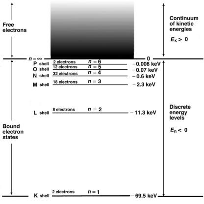
A simplified energy level diagram for tungsten, a typical multi-electron atom of importance in medical physics for its use as target material in x-ray tubes, is shown in Fig. 2.7. The K, L, M, and N shells are completely filled with their normal allotment of electrons (2n2), the O shell has 12 electrons and the P shell has 2 electrons.

The n > 1 shells are actually split into subshells, as discussed in Sect. 3.1.1. In Fig. 2.7 the fine structure of shells is represented by only one energy level that is equal to the average energy of all subshells for a given n.

•A vacancy in a shell with a low quantum number n will result in highenergy transitions in the keV range referred to as x-ray transitions.

•A vacancy in a shell with a high quantum number n will result in relatively low-energy transitions (in the eV range) referred to as optical transitions.

72 2 Rutherford–Bohr Atomic Model

Table 2.5. Expressions for the radius, velocity, energy and wave-number of atomic structure according to Bohr’s one-electron model and Hartree’s multi-electron model

	One-electron atom	Multi-electron atom
	Bohr theory	Hartree approximation
		Ze (for n = 1) ≈ Z − 2
		Ze (for outer shell) ≈ n
Radius rn	rn = ao n2	rn = ao	n2
	Z	Zeff
	ao				ao
	r1 = Z	r1 = rK ≈
				Z−2
	˚	router shell ≈ nao
	ao = 0.53 A

Velocity υn	υn = αc Z
			n
	υ1 = αcZ
	α =	1
	137

υn = αc Zneff

υ1 = υK ≈ αc (Z − 2)

υouter shell ≈ αc

E

−

Z2

2

−

2

2

Energy En

Z

En =

Zeff

1 =

ER

En =

ER

n

ER

n

−

E1 = EK ≈ −ER(Z − 2)

ER = 13.6 eV

Eouter shell ≈ −ER

2

f −

1

f −

1

1

2

1

1

Wave-number k

k = R∞ Z

n2

ni2

k = R∞ Ze

n2

ni2

R∞ = 109 737 cm−

Ze (Kα) ≈ Z − 1

k (Kα) ≈ 43 R∞ (Z − 1)2

2.4.3 Periodic Table of Elements

The chemical properties of atoms are periodic functions of the atomic number Z and are governed mainly by electrons with the lowest binding energy, i.e., by outer shell electrons commonly referred to as valence electrons. The periodicity of chemical and physical properties of elements (periodic law) was first noticed by Dmitry Mendeleyev, who in 1869 produced a periodic table of the then-known elements.

Since Mendeleyev’s time the periodic table of elements has undergone several modifications as the knowledge of the underlying physics and chemistry expanded and new elements were discovered and added to the pool. However, the basic principles elucidated by Mendeleyev are still valid today.

In a modern periodic table of elements each element is represented by its chemical symbol and its atomic number. The periodicity of properties of

2.4 Multi-electron Atoms

73

Fig. 2.7. A simplified energy level diagram for the tungsten atom, a typical example of a multi-electron atom

elements is caused by the periodicity in electronic structure that follows the rules of the Pauli exclusion principle (see Sect. 2.4.1).

The periodic table of elements is now most commonly arranged in the form of 7 horizontal rows or periods and 8 vertical columns or groups. Elements with similar chemical and physical properties are listed in the same column.

The periods in the periodic table are of increasing length as follows:

•Period 1 has two elements: hydrogen and helium.

•Periods 2 and 3 have 8 elements each.

•Periods 4 and 5 have 18 elements each.

•Period 6 has 32 elements condensed into 18 elements and the series of 14 lanthanons with atomic numbers Z from 57 through 71 is listed separately. Synonyms for lanthanon are lanthanide, lanthanoid, rare earth, and rareearth element.

74 2 Rutherford–Bohr Atomic Model

•Period 7 is still incomplete and the series of 14 actinons with atomic numbers Z from 89 through 103 is listed separately. Synonyms for actinon are actinide and actinoid.

The groups in the periodic table are arranged into 8 distinct groups, each group split into subgroups A and B. Each subgroup has a complement of electrons in the outermost atomic shell (in the range from 1 to 8) that determines its valence, i.e., chemical property.

Table 2.6 gives a simplified modern periodic table of elements with atomic numbers Z ranging from 1 (hydrogen) to 109 (meitnerium). Several groups of elements have distinct names, such as alkali elements (group I.A), alkali earth elements (group II.A), halogens (group VII.A) and noble gases (group VIII.A). Elements of other groups are grouped into transition metals, non-transition metals, non-metals (including halogens of group VII.A), lanthanons and actinons.

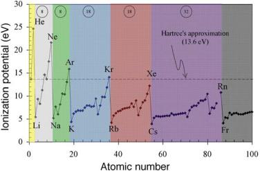
2.4.4 Ionization Potential of Atoms

The ionization potential (IP ) of an atom is defined as the energy required for removal of the least bound electron (i.e., the outer shell or valence electron) from the atom. The ER value predicted by Hartree [see (2.85)] is only an approximation and it turns out, as shown in Fig. 2.8, that the ionization potentials of atoms vary periodically with Z from hydrogen at 13.6 eV to a high value of 24.6 eV for helium down to about 4.5 eV for alkali elements that have only one outer shell (valence) electron.

The highest atomic ionization potential in nature is the ionization potential of the helium atom at 24.6 eV. In contrast, the ionization potential of a singly ionized helium atom (He+) can be calculated easily from the Bohr’s theory using (2.60) with Z = 2 and n = 1 to obtain an IP of 54.4 eV. This value is substantially higher than the IP for a helium atom because of the two-electron repulsive interaction that lowers the IP in the neutral helium atom.

A plot of the ionization potential IP against atomic number Z, shown in Fig. 2.8, exhibits peaks and valleys in the range from 4.5 eV to 24.6 eV, with the peaks occurring for noble gases (outer shell filled with 8 electrons) and valleys for alkali elements (one solitary electron in the outer shell). Note: the ionization potential of lead is a few eV in contrast to the ionization potential of the K shell in lead that is 88 keV.

2.5 Experimental Confirmation

of the Bohr Atomic Model

The Bohr atomic model postulates that the total energy of atomic electrons bound to the nucleus is quantized. The binding energy quantization follows

2.5 Experimental Confirmation of the Bohr Atomic Model

75

Table 2.6. Simplified periodic table of elements covering 109 known elements and consisting of 7 periods 8 groups, each group divided into subgroups A and B

76 2 Rutherford–Bohr Atomic Model

Fig. 2.8. Ionization potential (ionization energy) of atoms against atomic number Z. The noble gases that contain the most stable electronic configurations and the highest ionization potentials are identified, as are the alkali elements that contain the least stable electronic configurations and the lowest ionization potentials with only one valence electron in the outer shell. The circled numbers indicate the number of atoms in a given period

from the simple quantization of the electron angular momentum L = n . Direct confirmation of the electron binding energy quantization was obtained from the following three experiments:

1.Measurement of absorption and emission spectra of mono-atomic gases.

2.Moseley’s experiment.

3.Franck-Hertz experiment.

2.5.1 Emission and Absorption Spectra of Mono-Atomic Gases

In contrast to the continuous spectra emitted from the surface of solids at high temperatures, the spectra emitted by free excited atoms of gases consist of a number of discrete wavelengths. An electric discharge produces excitations in the gas, and the radiation is emitted when the gas atoms return to their ground state. Correct prediction of line spectra emitted or absorbed by monoatomic gases, especially hydrogen, serves as an important confirmation of the Bohr atomic model.

•The emission spectrum is measured by first collimating the emitted radiation by a slit, and then passing the collimated slit-beam through an optical prism or a di raction grating. The prism or grating breaks the beam into its wavelength spectrum that is recorded on a photographic

2.5 Experimental Confirmation of the Bohr Atomic Model

77

plate. Each kind of free atom produces its own characteristic emission line, making spectroscopy a useful complement to chemical analysis.

•In addition to the emission spectrum, it is also possible to study the absorption spectrum of gases. The experimental technique is similar to that used in measurement of the emission spectrum except that in the measurement of the absorption spectrum a continuous spectrum is made to pass through the gas under investigation. The photographic plate shows a set of unexposed lines that result from the absorption by the gas of distinct wavelengths of the continuous spectrum.

•For every line in the absorption spectrum of a given gas there is a corresponding line in the emission spectrum; however, the reverse is not true. The lines in the absorption spectrum represent transitions to excited states that all originate in the ground state. The lines in the emission spectrum, on the other hand, represent not only transitions to the ground state but also transitions between various excited states. The number of lines in an emission spectrum will thus exceed the number of lines in the corresponding absorption spectrum.

2.5.2 Moseley’s Experiment

Henry Moseley in 1913 carried out a systematic study of Kα x rays produced by all then-known elements from aluminum to gold using the Bragg technique of x-ray scattering from a crystalline lattice of a potassium ferrocyanide crystal. The characteristic Kα x rays (electronic transition from ni = 2 to nf = 1; see Sect. 3.1.1) were produced by bombardment of the targets with energetic electrons. The results of Moseley’s experiments serve as an excellent confirmation of the Bohr atomic theory.

From the relationship between the measured scattering angle φ and the known crystalline lattice spacing d (Bragg’s law: 2d sin φ = mλ, where m is

an integer) Moseley determined the wavelengths λ of Kα x rays for various

√

elements and observed that the ν where ν is the frequency (ν = c/λ) of the Kα x rays was linearly proportional to the atomic number Z. He then showed that all x-ray data could be fitted by the following relationship

√			√
	ν =		a(Z − b) ,			(2.86)

where a and b are constants.

√

The same ν versus Z behavior also follows from the Hartree-type approximation that in general predicts the following relationship for the wavenumber k

k =

1

=

ν

= R∞Ze2

1

1

(2.87)

−

λ

c

n2

n2

or

f

i

ν = Ze

(2.88)

cR∞

nf2

− ni2

.

√

1

1

78 2 Rutherford–Bohr Atomic Model

For Kα characteristic x rays, where ni = 2 and nf = 1, Hartree’s expression gives

	3			3
k(Kα) =		R∞Ze2	=		R∞(Z − 1)2 .	(2.89)
	4			4

Note that in the Kα emission Ze = Z − 1 rather than Ze = Z − 2 which is the Ze predicted by Hartree for neutral multi-electron atoms. In the Kα emission there is a vacancy in the K shell and the L-shell electron making the Kα transition actually sees an e ective charge (Z − 1)e rather than an e ective charge (Z − 2)e, as is the case for K-shell electrons in neutral atoms.

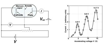
2.5.3 Franck-Hertz Experiment

Direct confirmation that the internal energy states of an atom are quantized came from an experiment carried out by James Franck and Gustav Hertz in 1914. The experimental set up is shown schematically in Fig. 2.9a.

•An evacuated vessel containing three electrodes (cathode, anode and plate) is filled with mercury vapor.

•Electrons are emitted thermionically from the heated cathode and accelerated toward the perforated anode by a potential V applied between cathode and anode.

•Some of the electrons pass through the perforated anode and travel to the plate, provided their kinetic energy upon passing through the perforated anode is su ciently high to overcome a small retarding potential Vret that is applied between the anode and the plate.

•The experiment involves measuring the electron current reaching the plate as a function of the accelerating voltage V .

(a)

(b)

Fig. 2.9. a Schematic diagram of the Franck-Hertz experiment; b Typical result of the Franck-Hertz experiment using mercury vapor