Radiation Physics for Medical Physiscists - E.B. Podgorsak

1.20 Important Relativistic Relationships

29

1.20.5 Taylor Expansion for Relativistic Kinetic Energy and Momentum

The Taylor expansion of a function f (x) about x = a is given as follows:

f (x) = f (a) + (x − a) dx x=a

df

(x

a)

2

2

f

(x

a)

n

d

n

f

d

+

−

+ . . . +

−

x=a

.

2!

dx2

n!

dxn

x=a

(1.52)

The Taylor expansion into a series given by (1.52) is particularly useful when one can neglect all but the first two terms of the series. For example, the first two terms of the Taylor expansion of the function f (x) = (1 ± x)n about x = 0 for x 1 are given as follows:

f (x) = (1 ± x)n ≈ 1 ± nx .

(1.53)

•The approximation of (1.53) is used in showing that, for small velocities

where υ c or υ/c 1, the relativistic kinetic energy EK of (1.45) transforms into the well-known classical relationship EK = moυ2/2

EK = E − Eo = moc2	1		− 1
		1 − υ2/c2

= moc2	(1 − υ2/c2)1/2 − 1
	1 − −	1		υ2		moυ2
≈ moc2					− . . . − 1 =		.	(1.54)
		2		c2		2

•Another example for the use of the Taylor expansion of (1.53) is the

classical relationship for the momentum p = moυ that, for υ c, i.e., (υ/c) 1, is obtained from the relativistic relationship for the momentum

given in (1.50) as follows:

p = c E2 − Eo2

= c mo2c4

1 − (υ2

/c2)

1

1

1

= c

1 − c2

− 1

m c2

υ2

−1

o

≈ moc

1 + c2

+ . . . − 1 = moυ .

υ2

− 1

(1.55)

1.20.6 Relativistic Doppler Shift

The speed of light emitted from a moving source is equal to c, a universal constant, irrespective of the source velocity. The energy as well as the wavelength and frequency of the emitted photons, on the other hand, depend on

30 1 Introduction to Modern Physics

the velocity of the moving source. The energy shift resulting from a moving source in comparison with the stationary source is referred to as the Doppler shift and the following conditions apply:

•When the source is moving toward the observer, the measured photon energy increases and the wavelength decreases (blue Doppler shift).

•When the source is moving away from the observer, the measured photon energy decreases and the wavelength increases (red Doppler shift).

1.21 Particle-Wave Duality:

Davisson–Germer Experiment

Both the electromagnetic radiation (photons) and particles exhibit a particlewave duality and both may be characterized with wavelength λ and momentum p related to one another through the following expression

	λ =	h		,	(1.56)
		p

where h is the Planck’s constant.

In relation to particles, (1.56) is referred to as the de Broglie relationship and λ is referred to as the de Broglie wavelength of a particle in honour of Louis de Broglie who in 1924 postulated the existence of matter waves.

The wave nature of the electron was confirmed experimentally by Clinton J. Davisson and Lester H. Germer in 1927 who set out to measure the energy of electrons scattered from a nickel target. The target was in the form of a regular crystalline alloy that was formed through a special annealing process. The beam of electrons was produced by thermionic emission from a heated tungsten filament. The electrons were accelerated through a relatively low variable potential di erence V that enabled the selection of the incident electron kinetic energy EK.

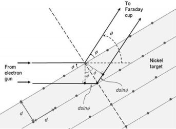
•Davisson and Germer discovered that for certain combinations of electron kinetic energies EK and scattering angles φ the intensity of scattered electrons exhibited maxima, similarly to the scattering of x rays from a crystal with a crystalline plane separation d that follows the Bragg relationship (see Fig. 1.5) with m an integer

2d sin φ = mλ .

(1.57)

•Similarly to Moseley’s work with Kα characteristic x rays (see Sect. 2.5.2), Davisson and Germer determined the wavelength λe of electrons from the measured scattering angle φ at which the electron intensity exhibited a maximum.

	• The measured		λe agreed			well with		wavelengths	calculated from the
	de Broglie relationship
	h		=	h	=		2π c
	λe =					√		,	(1.58)
		p		meυ
							2mec2eV

1.22 Matter Waves

31

Fig. 1.5. Davisson–Germer experiment of elastic electron scattering on a nickel single crystal target. The electrons are produced in an electron gun and scattered by the nickel crystalline structure that has an atom spacing d and acts as a reflection grating. The maximum intensity of scattered electrons occurs as a result of constructive interference from electron matter waves following the Bragg relationship of (1.57)

where υ is the velocity of electrons determined from the classical kinetic energy relationship EK = meυ2/2 = eV with V the applied potential.

The experimentally determined particle-wave duality suggests that both the particle model and the wave model can be used for particles as well as for photon radiation. However, for a given measurement only one of the two models will apply. For example, in the case of photon radiation, the Compton e ect is explained with the particle model, while the di raction of x rays is explained with the wave model. On the other hand, the charge-to-mass ratio e/me of the electron implies a particle phenomenon, while the electron di raction suggests wave-like behavior.

1.22 Matter Waves

Associated with any particle is a matter wave, as suggested by the de Broglie relationship of (1.56). This matter wave is referred to as the particle’s wave function Ψ (z, t) for one-dimensional problems or Ψ (x, y, z, t) for threedimensional problems and contains all the relevant information about the particle. Quantum mechanics or wave mechanics, developed by Erwin Schr¨o- dinger (wave mechanics) and Werner Heisenberg (matrix mechanics) between

32 1 Introduction to Modern Physics

1925 and 1929, is a branch of physics that deals with the properties of wave functions as they pertain to particles, nuclei, atoms, molecules and solids.

1.22.1 Introduction to Wave Mechanics

The main characteristics of wave mechanics are as follows:

•The theory has general application to microscopic systems and includes Newton’s theory of macroscopic particle motion as a special case in the macroscopic limit.

•The theory specifies the laws of wave motion that the particles of any microscopic system follow.

•The theory provides techniques for obtaining the wave functions for a given microscopic system.

•It o ers means to extract information about a particle from its wave function.

The main attributes of wave functions Ψ (z, t) are:

•Wave functions are generally but not necessarily complex and contain the imaginary number i.

•Wave functions cannot be measured with any physical instrument.

•Wave functions serve in the context of Schr¨odinger’s wave theory but contain physical information about the particle they describe.

•Wave functions must be single-valued and continuous functions of z and t to avoid ambiguities in predictions of the theory.

The information on a particle can be extracted from a complex wave function Ψ (z, t) through a postulate proposed by Max Born in 1926 relating the probability density dP (z, t)/dz in one dimension with the wave function Ψ (z, t) as follows:

dP (z, t)/dz = Ψ (z, t)	·	Ψ (z, t) .	(1.59)

Similarly we can relate the probability density dP (x, y, z, t)/dV in three dimensions with the wave function Ψ (x, y, z, t) as

dP (x, y, z, t)/dV = Ψ (x, y, z, t)	·	Ψ (x, y, z, t) ,	(1.60)

where Ψ is the complex conjugate of the wave function Ψ .

The probability density is real, non-negative and measurable. In onedimensional wave mechanics, the total probability of finding the particle somewhere along the z axis in the entire range of the z axis is equal to one, if the particle exists. We can use this fact to define the following normalization condition

+∞	(z, t)		+∞
	dP	dz =		Ψ (x, y, z, t)Ψ (x, y, z, t)dz = 1 .	(1.61)
	dz

−∞

−∞

1.22 Matter Waves

33

Similarly, in three-dimensional wave mechanics, the normalization expression is written as

+∞	(z, t)	+∞ +∞ +∞
	dP	dV =	Ψ (x, y, z, t)Ψ (x, y, z, t)dxdydz = 1 ,
	dV
−∞		−∞ −∞ −∞

(1.62)

where the volume integral extends over all space and represents a certainty that the particle will be found (unit probability). Any one-dimensional wave function Ψ (z, t) that satisfies (1.61) is said to be normalized. Similarly, any three-dimensional wave function Ψ (x, y, z) that satisfies (1.62) is also said to be normalized.

While the normalization condition expresses certainty that a particle, if it exists, will be found somewhere, the probability that the particle will be found in any interval a ≤ z ≤ b is obtained by integrating the probability density Ψ · Ψ from a to b as follows:

P = a	b
	Ψ · Ψ dV .	(1.63)

1.22.2 Quantum-Mechanical Wave Equation

The particulate nature of photons and the wave nature of matter are referred to as the wave-particle duality of nature. The waves associated with matter are represented by the wave function Ψ (x, y, z, t) that is a solution to a quantum mechanical wave equation. This wave equation cannot be derived directly from first principles of classical mechanics; however, it must honor the following four conditions:

1.It should respect the de Broglie postulate relating the wavelength λ of the wave function with the momentum p of the associated particle: p = h/λ = k, where k is the wave number defined as k = 2π/λ.

2.It should respect the Planck’s law relating the frequency ν of the wave function with the total energy E of the particle: E = hν = ω.

3.It should respect the relationship expressing the total energy E of a particle of mass m as a sum of the particle’s kinetic energy EK = p2/(2m) and potential energy V , i.e.,

E =	p2
		+ V .	(1.64)
	2m

4.It should be linear in Ψ (z, t) which means that any arbitrary linear combination of two solutions for a given potential energy V is also a solution to the wave equation.

While the wave equation cannot be derived directly, we can determine it for a free particle in a constant potential and then generalize the result to

34 1 Introduction to Modern Physics

other systems and other potential energies. The free particle wave function Ψ (z, t) can be expressed as follows:

Ψ (z, t) = Cei(kz−ωt) ,

(1.65)

where (kz − ωt) is the phase of the wave with k = 2π/λ the wave number and ω = 2πν the angular frequency of the wave.

We now determine the partial derivatives ∂/∂x and ∂/∂t of the wave function to obtain

∂Ψ (z, t)			= ikCei(kz−ωt)			= ikΨ (z, t) = i	p	Ψ (z, t)			(1.66)
	∂z
and
∂Ψ (z, t)			= −iωCei(kz−ωt) = −iωΨ (z, t) = −i						E	Ψ (z, t) .	(1.67)
	∂t
Equation (1.66) can now be written as follows:
pΨ (z, t) = −i				∂
					Ψ (z, t)						(1.68)
				∂z

where (−i ∂/∂z) is a di erential operator for the momentum p. Similarly we can write (1.67) as

	EΨ (z, t) = i	∂	Ψ (z, t) ,	(1.69)
		∂t

where (i ∂/∂t) is a di erential operator for the total energy E.

Equations (1.68) and (1.69) suggest that multiplying the wave function Ψ (z, t) by a given physical quantity, such as p and E in (1.68) and (1.69) has the same e ect as operating on Ψ (z, t) with an operator that is associated with the given physical quantity. As given in (1.64), the total energy E of the particle with mass m is the sum of its kinetic and potential energies.

If we now replace p and E in (1.64) with their respective operators, given in (1.68) and (1.69), we obtain

	2 ∂2				∂		(1.70)
−				+ V = i		.
	2m		∂z2		∂t

Equation (1.70) represents two new di erential operators; the left hand side operator is referred to as the hamiltonian operator [H], the right hand side operator is the operator for the total energy E. When the two operators of (1.70) are applied to a free particle wave function Ψ (z, t) we get

−	2 ∂2Ψ (z, t)				+ V Ψ (z, t) = i	∂Ψ (z, t)		(1.71)
							.
	2m		∂z2			∂t

Equation (1.71) was derived for a free particle moving in a constant potential V ; however, it turns out that the equation is valid in general for any potential energy V (z, t) and is referred to as the time-dependent Schr¨odinger equation with V (z, t) the potential energy describing the spatial and temporal dependence of forces acting on the particle of interest. The time-dependent

1.22 Matter Waves

35

Schr¨odinger equation is thus in the most general three dimensional form written as follows:

	2		∂Ψ (x, y, z, t)
−		2Ψ (x, y, z, t) + V (x, y, z, t)Ψ (x, y, z, t) = i		.
	2m		∂t

(1.72)

1.22.3 Time-Independent Schr¨odinger Equation

In most physical situations the potential energy V (z, t) only depends on z, i.e., V (z, t) = V (z) and then the time-dependent Schr¨odinger equation can be solved with the method of separation of variables.

The wave function Ψ (z, t) is written as a product of two functions ψ(z) and T (t), one depending on the spatial coordinate z only and the other depending on the temporal coordinate t only, i.e.,

Ψ (z, t) = ψ(z)T (t) .

(1.73)

Inserting (1.73) into the time-dependent wave equation given in (1.71) and dividing by ψ(z)T (t) we get

	2 1 ∂2ψ(z)						1
−							+ V (z) = i
	2m		ψ(z)		∂z2			T (t)

	∂T (t)	.	(1.74)
	∂t

Equation (1.74) can be valid in general only if both sides, the left hand side that depends on z only and the right hand side that depends on t only, are equal to a constant, referred to as the separation constant Λ. We now have two ordinary di erential equations: one for the spatial coordinate z and the other for the temporal coordinate t given as follows:

−		2 d2ψ(z)					+ V (z)ψ(z) = Λψ(z)		(1.75)
		2m		dz2
and
dT (t)					iΛ
				= −				T (t) .	(1.76)
	dt
The solution to the temporal equation is
T (t) = e−i Λ t							,		(1.77)

representing a simple oscillatory function of time with angular frequency ω = Λ/ . According to de Broglie and Planck the angular frequency must also be given as E/ , where E is the total energy of the particle.

We can now conclude that the separation constant Λ equals the total particle energy E and obtain from (1.76) the following solution to the temporal

equation
T (t) = e−i E t = e−iωt ,	(1.78)
where we used Planck’s relationship E	= ω.

36	1 Introduction to Modern Physics
	Recognizing that Λ = E we can write (1.75) as
	−	2 d2ψ(z)			+ V (z)ψ(z) = Eψ(z)	(1.79)
		2m		dz2

and obtain the so-called time-independent Schr¨odinger wave equation for the potential V (z).

The essential problem in quantum mechanics is to find solutions to the time-independent Schr¨odinger equation for a given potential energy V , generally only depending on spatial coordinates. The solutions are given in the form of:

1.Physical wave functions ψ(x, y, z) referred to as eigenfunctions.

2.Allowed energy states E referred to as eigenvalues.

The time-independent Schr¨odinger equation does not include the imaginary number i and its solutions, the eigenfunctions, are generally not complex. Since only certain functions (eigenfunctions) provide physical solutions to the time-independent Schr¨odinger equation, it follows that only certain values of E referred to as eigenvalues are allowed. This results in discrete energy values for physical systems and in energy quantization.

Many mathematical solutions are available as solutions to wave equations. However, to serve as a physical solution, an eigenfunction ψ(z) and its derivative dψ/dz must be: (1) finite, (2) single valued, and (3) continuous.

Corresponding to each eigenvalue En is an eigenfunction ψn(z) that is a solution to the time-independent Schr¨odinger equation for the potential Vn(z). Each eigenvalue is also associated with a corresponding wave function Ψ (z, t) that is a solution to the time-dependent Schr¨odinger equation and can be expressed as

Ψ (z, t) = ψ(z)e−i E t .

(1.80)

1.22.4 Measurable Quantities and Operators

As the term implies, a measurable quantity is any physical quantity of a particle that can be measured. Examples for measurable quantities are: position z, momentum p, kinetic energy EK, potential energy V , total energy E, etc.

In quantum mechanics an operator is associated with each measurable quantity. The operator allows for a calculation of the average (expectation) value of the measurable quantity, provided that the wave function of the particle is known.

¯

The expectation value (also referred to as the average or mean value) Q of a physical quantity Q, such as position z, momentum p, potential energy V , and total energy E of a particle is determined as follows provided that the particle’s wave function Ψ (z, t) is known

¯ (z, t)[Q]Ψ (z, t)dz , (1.81)

Q = Ψ

1.23 Uncertainty Principle

37

Table 1.5. Several measurable quantities and their associated operators used in quantum mechanics

Measurable quantity

Symbol

Associated operator

Symbol

Position

z

z

[z]

Momentum

p

−i

∂

[p]

∂z

Potential energy

V

V

[V ]

Kinetic energy

EK

−

2 ∂2

[EK]

2m

∂z2

Hamiltonian

2

∂2

H

−

+ V

[H]

2m

∂z2

Total energy

E

i

∂

[E]

∂t

where [Q] is the operator associated with the physical quantity Q. A listing of most common measurable quantities in quantum mechanics and their associated operators is given in Table 1.5.

The quantum uncertainty ∆Q for any measurable quantity Q is given as

∆Q =				− Q¯2		(1.82)
			Q2		,
¯2
	is the square of the expectation value of the quantity Q and Q							2	is
where Q

the expectation value of Q2.

•When ∆Q = 0, the measurable quantity Q is said to be sharp and all measurements of Q yield identical results.

•In general ∆Q > 0, and repeated measurements result in a distribution of measured points.

1.23 Uncertainty Principle

In classical mechanics the act of measuring the value of a measurable quantity does not disturb the quantity; therefore, the position and momentum of an object can be determined simultaneously and precisely. However, when the size of the object diminishes and approaches the dimensions of microscopic particles, it becomes impossible to determine with great precision at the same instant both the position and momentum of particles or radiation nor is it possible to determine the energy of a system in an arbitrarily short time interval.

Werner Heisenberg in 1927 proposed the uncertainty principle that limits the attainable precision of measurement results. The uncertainty principle covers two distinct components:

1.The momentum-position uncertainty principle deals with the simultaneous measurement of the position z and momentum pz of a particle and

38 1 Introduction to Modern Physics

limits the attainable precision of z and pz measurement to the following

∆z∆pz ≥		,	(1.83)
	2

where ∆z is the uncertainty on z and ∆pz is the uncertainty on pz. There are no limits on the precision of individual z and pz measurements. However, in a simultaneous measurement of z and pz the product of the two uncertainties cannot be smaller than /2, where is the reduced Planck’s constant ( = h/2π). If z is known precisely (∆z = 0), then we cannot know pz , since (∆pz = ∞). The reverse is also true: if pz is known exactly (∆pz = 0), then we cannot know z, since ∆z = ∞.

2.The other component (energy-time uncertainty principle) deals with the measurement of the energy E of a system and the time interval ∆t required for the measurement. Similarly to the (∆z, ∆pz ) situation, Heisenberg uncertainty principle states the following

∆E∆t ≥		,	(1.84)
	2

where ∆E is the uncertainty in the energy determination and ∆t is the time interval taken for the measurement.

Classical mechanics sets no limits on the precision of measurement results and allows a deterministic prediction of the behavior of a system in the future. Quantum mechanics, on the other hand, limits the precision of measurement results and thus allows only probabilistic predictions of the system’s behavior in the future.

1.24 Complementarity Principle

In 1928 Niels Bohr proposed the principle of complementarity postulating that any atomic scale phenomenon for its full and complete description requires that both its wave and particle properties be considered and determined, since the wave and particle models are complementary. This is in contrast to macroscopic scale phenomena where particle and wave characteristics (e.g., billiard ball vs. water wave) of the same macroscopic phenomenon are mutually incompatible rather than complementary.

Bohr’s principle of complementarity is thus valid only for atomic size processes and asserts that these processes can manifest themselves either as waves or as particles (corpuscules) during a given experiment, but never as both during the same experiment. However, to understand and describe fully an atomic scale physical process the two types of properties must be investigated with di erent experiments, since both properties complement rather than exclude each other.

The most important example of this particle-wave duality is the photon, a mass-less particle characterized with energy, frequency and wavelength. How-