Radiation Physics for Medical Physiscists - E.B. Podgorsak

2.6 Schr¨odinger Equation for the Ground State of Hydrogen

79

•With an increasing potential V the current at the plate increases with V until, at a potential of 4.9 V, it abruptly drops, indicating that some interaction between the electrons and mercury atoms suddenly appears when the electrons attain a kinetic energy of 4.9 eV. The interaction was interpreted as an excitation of mercury atoms with a discrete energy of 4.9 eV; the electron raising an outer shell mercury electron to its first excited state and, in doing so, losing its kinetic energy and its ability to overcome the retarding potential Vret between the anode and the plate.

•The sharpness of the current drop at 4.9 V indicates that electrons with energy below 4.9 eV cannot transfer their energy to a mercury atom, substantiating the existence of discrete energy levels for the mercury atom.

•With voltage increase beyond 4.9 V the current reaches a minimum and then rises again until it reaches another maximum at 9.8 V, indicating that some electrons underwent two interactions with mercury atoms. Other maxima at higher multiples of 4.9 V were observed with careful experiments. Typical experimental results are shown in Fig. 2.9b.

•In contrast to the minimum excitation potential of the outer shell electron

in mercury of 4.9 eV, the ionization potential of mercury is 10.4 eV.

• ˚

A further investigation showed a concurrent emission of 2536 A ultraviolet rays that, according to Bohr model, will be emitted when the mercury atom reverts from its first excited state to the ground state through a

4.9 eV optical transition.

•The photon energy Eν = 4.9 eV is given by the standard relationship

Eν = hν = 2π c/λ ,

(2.90)

from which the wavelength of the emitted photon can be calculated as

	2π		c		2π 197.4 × 10	6	eV 10	−5 ˚
λ =				=				A	= 2536 A˚ .	(2.91)
	Eν				4.9 eV

˚

Ultraviolet photons with a wavelength of 2536 A were actually observed accompanying the Franck-Hertz experiment, adding to the measured peaks in the current versus voltage diagram of Fig. 2.9b another means for the confirmation of the quantization of atomic energy levels.

2.6 Schr¨odinger Equation

for the Ground State of Hydrogen

In solving the Schr¨odinger equation for a hydrogen or hydrogen-like oneelectron atom, a 3-dimensional approach must be used to account for the electron motion under the influence of a central force. The Coulomb potential binds the electron to the nucleus and the coordinate system is chosen such that its origin coincides with the center of the nucleus. To account for the motion of the nucleus we use the reduced mass µ of (2.66) rather than the pure electron rest mass me in the calculation.

80 2 Rutherford–Bohr Atomic Model

The time-independent Schr¨odinger wave equation was given in (1.79) as

−	2
	2µ 2ψ + V (r)ψ = Eψ ,	(2.92)

where

V (r) is the potential energy of the particle,

Eis the total energy of the particle

2	is the Laplacian operator in Cartesian, cylindrical or spherical coor-
	dinates,

µis the reduced mass of the electron/proton system given in (2.66).

For the hydrogen atom, the potential V (r) is represented by the sphericallysymmetric Coulomb potential as follows:

V (r) = −	1	e2			(2.93)
				.
	4πεo		r

The Schr¨odinger wave equation is separable in spherical coordinates (r, θ, φ) and for the hydrogen atom it is written by expressing the Laplacian operator in spherical coordinates as follows:

2

1 ∂

∂

1 ∂

∂

1 ∂2

−

r2

+

sin θ

+

2µ

r2

∂r

∂r

r2 sin θ

∂θ

∂θ

r2 sin2 θ

∂φ2

ψ(r, θ, φ) −

e2 1

ψ(r, θ, φ) = Eψ(r, θ, φ) ,

(2.94)

4πεo

r

with (r, θ, φ) the spherical coordinates of the electron.

The boundary conditions stipulate that |ψ|2 must be an integrable function. This implies that the wave function ψ(r, θ, φ) vanishes as r → ∞, i.e.,

the condition that lim ψ(r, θ, φ) = 0 must hold.

r→∞

Equation (2.94) can be solved with the method of separation of variables by expressing the function ψ(r, θ, φ) as a product of three functions: R(r), Θ(θ), and Φ(φ); each of the three functions depends on only one of the three

spherical variables, i.e.,
ψ(r, θ, φ) = R(r)Θ(θ)Φ(φ) .	(2.95)

Inserting (2.95) into (2.94) and dividing by R(r)Θ(θ)Φ(φ) we get the

following expression

−

2

1 1 ∂

r2

∂R

+

1 1 ∂

sin θ

∂Θ

+

1 1 ∂2Φ

2µ

r2

R

∂r

∂r

r2 sin θ

Θ

∂θ

∂θ

r2 sin2 θ

Φ

∂φ2

−

e2 1

= E ,

(2.96)

4πεo

r

Separation of variables then results in the following three ordinary di erential equations

d2Φ	= −m Φ ,	(2.97)
dφ2

2.6

Schr¨odinger Equation for the Ground State of Hydrogen

81

1

d

dΘ

m2Θ

−

sin θ

+

= ( + 1)Θ ,

(2.98)

sin θ

dθ

dθ

sin2 θ

and

1 d

dR

2µ

e2

R

r2

+

E +

R = ( + 1)

,

(2.99)

r2

dr

dr

2

4πεo

r2

with separation constants m and ( + 1), where m and are referred to as the magnetic and orbital quantum numbers, respectively.

Equation (2.99) for R(r) gives physical solutions only for certain values of the total energy E. This indicates that the energy of the hydrogen atom is quantized, as suggested by the Bohr theory, and predicts energy states that are identical to those calculated for the Bohr model of the hydrogen atom. The energy levels En calculated from the Schr¨odinger wave equation, similarly to those calculated for the Bohr atom, depend only on the principal quantum number n; however, the wave function solutions depend on three quantum numbers: n (principal), (orbital) and m (magnetic). All quantum

numbers are integers governed by the following rules:
n = 1, 2, 3 . . . , = 0, 1, 2, . . . n − 1,
m = − , − + 1, . . . ( − 1), .	(2.100)

Equation (2.94) is generally quite complex yielding wave functions for the ground state n = 1 of the hydrogen atom as well as for any of the excited states with associated values of quantum numbers and m .

The ground state of the hydrogen atom can be calculated in a simple fashion as follows. Since V (r) is spherically symmetric, we assume that solutions to the Schr¨odinger equation for the ground state of hydrogen will be spherically symmetric which means that the wave function ψ(r, θ, φ) does not depend on θ and ϕ, it depends on r alone, and we can write for the spherically symmetric solutions that ψ(r, θ, φ) = R(r).

The Schr¨odinger equation then becomes significantly simpler and after some rearranging of terms it is given as follows:

d2R(r)

2

dR(r)

µ e2

2µE

+

+

R(r) +

R(r) = 0 . (2.101)

dr2

r

dr

2

4πεo

2

We can now simplify the Schr¨odinger equation further by recognizing that for large r the (1/r) term will be negligible and we obtain

	2R(r)			µE
	d		− −	2	R(r) ≈ 0 .	(2.102)
	dr2			2

Next we define the constant −2µE/ 2 as λ2 and recognize that the total energy E1 for the ground state of hydrogen will be negative

λ2 = −	2µE1	.	(2.103)
	2

82 2 Rutherford–Bohr Atomic Model

The simplified Schr¨odinger equation is now given as follows:

d2R(r)	− λ2R(r) = 0 .	(2.104)
dr2

Equation (2.104) is recognized as a form of the Helmholtz di erential equation in one dimension that leads to exponential functions for λ2 > 0, to a linear function for λ = 0, and to trigonometric functions for λ < 0. Since the total energy E is negative for bound states in hydrogen, λ2 is positive and the solutions to (2.104) will be exponential functions. The simplest exponential solution is

R(r) = Ce−λr ,							(2.105)
with the first derivative expressed as
	dR(r)	=	−	λCe−λr =	−	λR(r) .	(2.106)
	dr

The second derivative of the function R(r) of (2.105) is given as follows:

	d2R(r)		= λ2Ce−λr = λ2R(r) .	(2.107)
	dr2

Inserting (2.105) and (2.107) into (2.104) shows that (2.105) is a valid solution to (2.104). We now insert (2.105), (2.106) and (2.107) into (2.101) and get the following expression

2		−λ +	µ e2			R(r) +	2µE	1
λ2R(r) +									R(r) = 0 .	(2.108)
	r		2		4πεo		2

The first and fourth terms of (2.108) cancel out because λ2 is defined as (−2µE1/ 2) in (2.103). Since (2.108) must be valid for any ψ(r), the term in curly brackets equals zero and provides another definition for the constant λ as follows:

λ =	µ e2			=	µc2		e2	.	(2.109)
	2 4πεo
					( c)2 4πεo

We recognize (2.109) for λ as the inverse of the Bohr radius ao that was given in (2.58). Therefore, we express 1/λ as follows:

1	= ao =	( c)2 4πεo			˚
λ		µc2		e2	= 0.5292 A .	(2.110)

Combining (2.103) and (2.109) for the constant λ we now express the ground state energy E1 as

	1	2 1					1		e2		2 µc2
E1 = −						= −							= −13.61 eV .	(2.111)
	2		µ		ao2		2		4πεo			( c)2

The wave function R(r) for the ground state of hydrogen is given in (2.105) in general terms with constants C and λ. The constant λ was established in (2.110) as the inverse of the Bohr radius ao; the constant C we determine from

2.6 Schr¨odinger Equation for the Ground State of Hydrogen

83

the normalization condition of (1.62) that is given by the following expression

	2
	|ψ(r)| dV = 1 ,	(2.112)

with the volume integral extending over all space.

The constant C is determined after inserting ψ(r, θ, φ) = R(r) given by (2.105) into (2.112) to obtain

	2	dV = C2	2π π ∞			e− ao r2dφ sin θdθdr
	|ψ(r)|		0	0	0
						2r
		= 4πC2		∞			4ao3 = 1 ,		(2.113)
				0	r2e− ao dr = 4πC2
						2r	1

where the last integral over r is determined from the following recursive formula

	xneaxdx = a xneax − a			xn−1eaxdx .	(2.114)
	1		n

The integral over r in (2.113) is equal to 1/(4a3o) and the constant C is now given as follows:

C = π−1/2ao−3/2 ,

(2.115)

resulting in the following expression for the wave function R(r) for the ground state of the hydrogen atom

	1		e−	r
ψn, ,m	(r, θ, φ) = ψ100 = R1(r) =			ao	.	(2.116)
	π1/2ao3/2

The probability density of (1.60) can now be modified to calculate the radial probability density dP/dr as follows:

	dP	= ψ (r, θ, φ)ψ(r, θ, φ) = |ψ(r, θ, φ)|2	(2.117)
dV
and
dP		= 4πr2 |ψ(r, θ, φ)|2 ,	(2.118)
	dr

since dV = 4πr2dr for the spherical symmetry governing the ground state (n = 1) of the hydrogen atom.

The radial probability density dP/dr for the ground state is given as follows, after inserting (2.116) into (2.118):

dP		=	2		e− ao .	(2.119)
			4r3
					2r
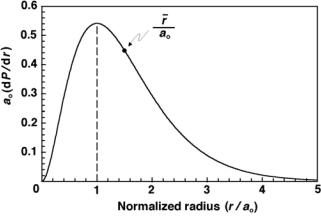
	dr			ao		given as 4(r/ao)2 exp(−2r/ao) against
A plot		of	unit-less ao(dP/dr)

(r/ao) for the ground state of the hydrogen atom is shown in Fig. 2.10. The following observations can be made based on data shown in Fig. 2.10:

84 2 Rutherford–Bohr Atomic Model

Fig. 2.10. The radial probability density multiplied with the Bohr radius ao against normalized radius r for the ground state electron of hydrogen

1.dP/dr = 0 for r = 0 and r = ∞.

2.dP/dr reaches its maximum at r = ao highlighting Schr¨odinger’s theory prediction that the ground state electron in hydrogen is most likely to be

found at r = ao where ao is the Bohr radius given in (2.58). One can also obtain this result by calculating d2P/dr2 and setting the result equal to zero at r = rmax. Thus, the most probable radius rp for the electron in the ground state of hydrogen is equal to ao.

3.Contrary to Bohr theory that predicts the electron in a fixed orbit with

r = ao, Schr¨odinger’s theory predicts that there is a finite probability for the electron to be anywhere between r = 0 and r = ∞. However, the most probable radius for the electron is r = ao.

To illustrate Schr¨odinger’s theory better a few simple calculations will now be made for the ground state of hydrogen:

1.The probability that the orbital electron will be found inside the first Bohr radius ao is calculated by integrating (2.119) from r = 0 to r = ao to get

4

ao

4e−2r/ao

aor2

a2r

a3

r=ao

−

r=0

0

−

−

ao3

ao3

2

2

4

P =

r2e−2r/ao dr =

o

o

r=ao

= − e−2r/ao 2

ao

+ 2

ao + 1 r=0

= 1 − 5e−2 = 0.323

r

2

r

(2.120)

2.6 Schr¨odinger Equation for the Ground State of Hydrogen

85

2.The probability that the orbital electron will be found with radius ex-

ceeding aois similarly calculated by integrating (2.119) from r = ao to r = ∞

4

ao

4e−2r/ao

aor2

a2r

a3

r=∞

0

−

−

−

r=ao

ao3

ao3

2

2

4

P =

r2e−2r/ao dr =

o

o

2

r=∞

= − e−2r/ao

2

ao

+ 2

= 5e−2

= 0.677

ao + 1 r=ao

r

r

(2.121)

3.The probability that the orbital electron will be found inside the nucleus (proton) is calculated by integrating (2.119) from r = 0 to r = R where R

is the proton radius estimated from (1.14) as R ≈ 1.2 fm. Using R/ao = 2.4 × 10−5 we get the following probability

4

ao

4e−2r/ao

aor2

a2r

a3

r=R

0

−

r=0

−

−

ao3

ao3

2

2

4

P =

r2e−2r/ao dr =

o

o

r=R

= − e−2r/ao

2 ao

+ 2

ao + 1 r=0

r

2

r

= 1 − e−2R/ao

2 ao

2

+ 2

ao + 1 ≈ 2.3 × 10−9

R

R

(2.122)

4. The average electron radius r¯ is calculated from (1.81) to get

r¯ =

2

∞

r

e

dr =

4

2 ao

(2.123)

r [R(r)] dV = ao3

0

16a03 =

4

3

− ao

4ao3!

3

2r

The most probable radius rp = ao and the /average radius r¯ = 1.5ao are not identical because the radial probability density distribution is not symmetrical about its maximum at ao, as shown in Fig. 2.10. As calculated in (2.120) and (2.121), the area under the dP/dr curve between r = 0 and r = ao is exactly one half the area under the curve between r = ao and r = ∞. As shown in (2.122), the probability for the electron to venture inside the proton nucleus is very small but not negligible.

Linear Accelerator Waveguide

The photograph on the next page shows a cut-away view of a simple standing wave accelerating waveguide used in a medical linear accelerator to accelerate electrons to a kinetic energy of 6 MeV that corresponds to a velocity of 99.7% of the speed of light in vacuum.

In contrast to x-ray tubes that use an electrostatic potential between the anode (target) and the cathode (filament) for acceleration of electrons to a given kinetic energy of the order of 100 keV, a medical linear accelerator (linac) uses an accelerating waveguide in which electrons are accelerated with electromagnetic fields to much higher kinetic energies in the range from 4 MeV to 25 MeV.

Waveguides are evacuated or gas-filled structures of rectangular or circular cross sections used in transmission of microwaves. Two types of waveguides are used in linacs: radiofrequency power transmission waveguides (usually gas-filled) and accelerating waveguides (always evacuated). The power transmission waveguides transmit the radiofrequency power from the power source to the accelerating waveguide in which electrons are accelerated. The electrons are accelerated in the accelerating waveguide by means of energy transfer from the high power microwave field that is set up in the accelerating waveguide and produced by the radiofrequency power generator.

The simplest accelerating waveguide is obtained from a cylindrical uniform waveguide by adding a series of irises (disks) with circular holes at the center and placed at equal distances along the uniform waveguide. These irises divide the waveguide into a series of cylindrical cavities that form the basic structure of the accelerating waveguide. The phase velocity of radiofrequency in a uniform waveguide exceeds that of the speed of light in vacuum and one of the roles of the irises is to slow down the radiofrequency below the speed of light to allow electron acceleration. The irises also couple the cavities, distribute microwave power from one cavity to another, and provide a suitable electric field pattern for acceleration of electrons in the accelerating waveguide.

The waveguide cavities are clearly visible on the photograph of the waveguide; the accelerating cavities are on the central axis of the waveguide, the radiofrequency coupling cavities are o side. The source of electrons (electron gun) is on the left, the x-ray target on the right, both permanently embedded into the waveguide structure. The electron gun is a simple electrostatic accelerator that produces electrons thermionically in a heated filament and accelerates them to a typical energy of 20 keV. The target is made of metal thicker than the 6 MeV electron range in the target material. The 6 MeV electrons are stopped in the target and a small portion of their energy is transformed into bremsstrahlung x rays that form a spectrum ranging in photon energies from 0 to 6 MeV and have an e ective energy of about 2 MeV. The bremsstrahlung x-ray beam produced by 6 MeV electrons striking a target is referred to as a 6 MV beam.

3 Production of X Rays

This chapter is devoted to a study of the production of the two known types of x rays: characteristic radiation and bremsstrahlung. Both types of x rays are important in medical physics, since both are used extensively in diagnostic imaging and in external beam radiotherapy. Characteristic x-rays are produced by electronic transitions in atoms triggered by vacancies in inner electronic shells of the absorber atom. Bremsstrahlung, on the other hand, is produced by Coulomb interactions between an energetic light charged particle and the nucleus of the absorber atom. Vacancies in electronic shells of atoms can be produced by various means such as Coulomb interactions, photon interactions, nuclear decay, positron annihilation and Auger e ect; however, x-rays used in medicine are produced only through Coulomb interactions of energetic electrons with orbital electrons and nuclei of an x-ray target.

This chapter provides a discussion of theoretical and practical aspects

ˇ

of x-ray production, briefly introduces Cerenkov radiation and synchrotron radiation, both of some interest in nuclear and medical physics, and concludes with a brief discussion of various accelerators of interest in medicine.

88 3 Production of X Rays

3.1 X-Ray Line Spectra (Characteristic Radiation)

A vacancy in an atomic shell plays an important role in physics and chemistry. Defined as an electron missing from the normal complement of electrons in a given atomic shell, a vacancy can be produced by eight di erent e ects or interactions ranging from various photon-atom interactions through charge particle-atom interactions to nuclear e ects. Depending on the nature and energy of the interaction, the vacancy may occur in the outer shell or in one of the inner shells of the atom. The list of the 8 e ects for production of shell vacancy in an atom is as follows:

1.Photoelectric e ect (see Sect. 7.5)

2.Compton scattering (see Sect. 7.3)

3.Triplet production (see Sect. 7.6.1)

4.Charged particle Coulomb interaction with an atom (see Sect. 5.3.1)

5.Internal conversion (see Sect. 8.9.3)

6.Electron capture (see Sect. 8.8.4)

7.Positron annihilation (see Sect. 7.6.7)

8.Auger e ect (see Sect. 3.1.2)

An atom with a vacancy in its inner shell is in a highly excited state and returns to its ground state through a series of electronic transitions. Electrons from higher atomic shells will fill the shell vacancies and the energy di erence in binding energies between the initial and final shell or sub-shell will be emitted from the atom in one of two ways:

1.Radiatively in the form of characteristic (fluorescent) radiation.

2.Non-radiatively in the form of Auger electrons, Coster-Kronig electrons or super Coster-Kronig electrons.

3.1.1 Characteristic Radiation

Radiative transitions result in emission of photons that are called characteristic radiation, since the wavelength λ and energy hν of the emitted photon are characteristic of the atom in which the photon originated. An older term, fluorescent radiation, is occasionally used to describe the characteristic photons. The set of radiative transition photons emitted from a given atom is referred to as the line spectrum of the atom. Charles G. Barkla is credited with the discovery of characteristic x rays.

Energy level diagrams for high atomic number x-ray targets are usually drawn using the n, , j and mj quantum numbers, as shown in Fig. 3.1. In addition to dependence on n (main structure), the energy level diagram also exhibits dependence on and j (fine structure). However, only certain allowed transitions, fulfilling specific selection rules, result in x rays. In Fig. 3.1 only transitions from the M and L to the K shell are shown; allowed transitions with solid lines and a forbidden transition with a dotted line.