Radiation Physics for Medical Physiscists - E.B. Podgorsak

4.5 Mass Angular Scattering Power for Electrons

139

In air the square of the spatial spread of the electron pencil beam, A2, is related to T /ρ and z, the thickness of the air layer from the pencil beam origin through the following expression

A2(z) =	T	ρz3			(4.69)
				.
	ρ		3

In deriving (4.69) the following assumptions are made:

1.Only small angle scattering events are considered.

2.The air layer z is much smaller than the electron range in air.

3.Secondary electrons, set in motion by the electron incident pencil beam, are ignored.

4.The bremsstrahlung contamination of the electron pencil beam is ignored.

Function A2(z) given in (4.69) is a linear function of z3 with the slope proportional to the mass angular scattering power T /ρ, which in turn is a function of electron beam kinetic energy EK through function τ given in (4.68). Thus, from a measurement of A2(z), the spatial spread of an electron pencil beam in air, at several distances z from the pencil beam origin, one first determines T /ρ through (4.69) and then determines the electron beam kinetic energy EK with data tabulated for air or data calculated for air from (4.68).

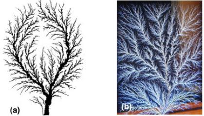
Lichtenberg Figures

Images on the next page are so-called Lichtenberg figures: in part (a) calculated using the fractal geometry technique and in part (b) produced by 10 MeV electrons deposited in a Lucite (acrylic) block.

The first Lichtenberg figures were actually two-dimensional patterns formed in dust on a charged plate in the laboratory of their discoverer, Georg Christoph Lichtenberg, an 18th century German physicist. The basic principles involved in the formation of these early figures are also fundamental to the operation of modern copy machines and laser printers.

Fractal geometry is a modern invention in comparison to the over 2000 year-old Euclidean geometry. Man-made objects usually follow Euclidean geometry shapes and are defined by simple algebraic formulas. In contrast, objects in nature often follow the rules of fractal geometry defined by iterative or recursive algorithms. Benoit B. Mandelbrot, a Polish-American mathematician is credited with introducing the term and techniques of fractal geometry during the 1970s. The most striking feature of fractal geometry is the so-called self-similarity implying that the fractal contains smaller components that replicate the whole fractal when magnified. In theory a fractal is composed of an infinite number of ever diminishing components, all of the same shape.

High-voltage electrical discharges on the surface or inside of insulating materials often result in Lichtenberg figures or patterns. Lucite is usually used as the medium for capturing the Lichtenberg figures, because it has an excellent combination of optical (it is transparent), dielectric (it is an insulator), and mechanical (it is strong, yet easy to machine) properties suitable for highlighting the Lichtenberg e ect. Electrons accelerated in a linear accelerator (linac) to a speed close to the speed of light in vacuum are made to strike a Lucite block. They penetrate into the block and come to rest inside the block. The electron space charge trapped in the block is released either spontaneously or through mechanical stress, and the discharge paths within the Lucite leave permanent records of their passage as they melt and fracture the plastic along the way. The charge exit point appears as a small hole at the surface of the Lucite block. Similar breakdown, albeit on a much larger scale, occurs during a lightning flash as the electrical discharge drains the highly charged regions within storm clouds; however, the discharge in air leaves behind no permanent record of the passage through air.

The fractal tree shown in (a) is a typical example of fractal geometry use in calculating the shape of a natural object. An example of a frozen Lichtenberg discharge in Lucite is shown in (b). The similarity between the calculated and the measured “tree” is striking.

(a)Courtesy of Prof. Volkhard Nordmeier, Technische Universit¨at, Berlin.

(b)Courtesy of Bert Hickman, Stoneridge Engineering, www.teslamania.com

5 Interactions of Charged Particles with Matter

In this chapter we discuss interactions of charged particle radiation with matter. A charged particle is surrounded by its Coulomb electric force field that interacts with orbital electrons (collision loss) and the nucleus (radiative loss) of all atoms it encounters as it penetrates into matter. The energy transfer from the charged particle to matter in each individual atomic interaction is generally small, so that the particle undergoes a large number of interactions before its kinetic energy is spent. Stopping power is the parameter used to describe the gradual loss of energy of the charged particle as it penetrates into an absorbing medium. Two classes of stopping powers are known: collision (ionization) stopping power that results from charged particle interaction with orbital electrons of the absorber and radiative stopping power that results from charged particle interaction with nuclei of the absorber.

Stopping powers play an important role in radiation dosimetry. They depend on the properties of the charged particle such as its mass, charge, velocity and energy as well as on the properties of the absorbing medium such as its density and atomic number. In addition to stopping powers, other parameters of charged particle interaction with matter, such as the range, energy transfer, mean ionization potential, and radiation yield, are also discussed in this chapter.

142 5 Interactions of Charged Particles with Matter

5.1 General Aspects of Stopping Power

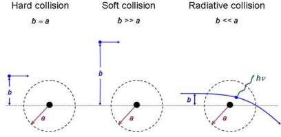
As a charged particle travels through an absorber, it experiences Coulomb interactions with the nuclei and the orbital electrons of the absorber atoms. These interactions can be divided into three categories depending on the size of the classical impact parameter b compared to the classical atomic radius a:

1.Coulomb force interaction of the charged particle with the external nuclear field (bremsstrahlung production) for b a.

2.Coulomb force interaction of the charged particle with orbital electron for b ≈ a (hard collision).

3.Coulomb force interaction of the charged particle with orbital electron for b a (soft collision).

Generally, the charged particle experiences a large number of interactions before its kinetic energy is expended. In each interaction the charged particle’s path may be altered (elastic or inelastic scattering) and it may lose some of its kinetic energy that will be transferred to the medium (collision loss) or to photons (radiative loss).

Radiative, hard and soft collisions are shown schematically in Fig. 5.1, with b the impact parameter and a the atomic radius.

•The rate of energy loss per unit of path length by a charged particle in a medium is called the linear stopping power (dE/dx).

•The stopping power is typically given in units MeV · cm2/g and then referred to as the mass stopping power S equal to the linear stopping power divided by the density ρ of the absorbing medium.

•The stopping power is a property of the material in which a charged particle propagates.

Fig. 5.1. Three di erent types of collisions of a charged particle with an atom, depending on the relative sizes of the impact parameter b and atomic radius a. Hard collision for b ≈ a; soft collision for b a; and radiative collision for b a

5.2 Radiative Stopping Power

143

Two types of stopping powers are known:

1.Radiative stopping power that results from charged particle Coulomb interaction with the nuclei of the absorber. Only light charged particles (electrons and positrons) experience appreciable energy losses through these interactions that are usually referred to as bremsstrahlung interactions.

2.Collision (ionization) stopping power that results from charged particle Coulomb interactions with orbital electrons of the absorber. Both heavy and light charged particles experience these interactions that result in energy transfer from the charged particle to orbital electrons, i.e., excitation and ionization of absorber atoms.

The total stopping power Stot for a charged particle of energy EK traveling through an absorber of atomic number Z is the sum of the radiative and collision stopping power, i.e.,

Stot = Srad + Scol .

(5.1)

5.2 Radiative Stopping Power

The rate of bremsstrahlung production by light charged particles (electrons and positrons) traveling through an absorber is expressed by the mass radiative stopping power Srad (in MeV · cm2/g) which is given as follows:

	Srad = NaσradEi ,	(5.2)
where
Na	is the number of atoms per unit mass: Na = N/m = NA/A,
σrad	is the total cross section for bremsstrahlung production given for various
	energy ranges in Table 5.1,
Ei	is the initial total energy of the light charged particle, i.e., Ei = EKi +
	mec2,
EKi	is the initial kinetic energy of the light charged particle.

Inserting σrad for non-relativistic particles from Table 5.1 into (5.2) we obtain the following expression for Srad:

2	2 NA
Srad = αre Z			BradEi ,	(5.3)
		A

where Brad is a slowly varying function of Z and Ei, also given in Table 5.1 and determined from σrad/(α re2Z2). The parameter Brad has a value of 16/3 for light charged particles in the non-relativistic energy range (EK mec2); about 6 at EK = 1 MeV; 12 at EK = 10 MeV; and 15 at EK = 100 MeV.

The mass radiative stopping power Srad is proportional to:

•(NAZ2/A), that, by virtue of Z/A ≈ 0.5 for all elements with the exception of hydrogen, indicates a proportionality with the atomic number of the absorber Z.

144 5 Interactions of Charged Particles with Matter

Table 5.1. Total cross section for bremsstrahlung production and parameter Brad for various ranges of electron kinetic energies

Energy range

σrad (cm2/nucleon)

Brad = σrad/(α re2Z2)

Non-relativistic				16	α re2Z2												16													(5.4)
				3														3
EKi	mec2
Relativistic			complicated power series														—													(5.5)
EKi ≈ mec2		mec2	8αre Z				ln	mec2 − 6									8		ln	mec2				−				6		(5.6)
mec2	EKi
High-relativistic			2			2				Ei					1							Ei						1
Extrememec2		αZ1/3			e			Z1/3				18									Z1/3				18
	relativistic		4αr2Z			2 ln		183				+		1			4		ln		183		+		1					(5.7)

EKi α Z1/3

•Total energy Ei (or kinetic energy EKi for EKi mec2)) of the light charged particle.

•Equation (5.3) was derived theoretically by Hans Bethe and Walter Heitler. Martin Berger and Stephen Seltzer have provided extensive tables of Srad for a wide range of absorbing materials

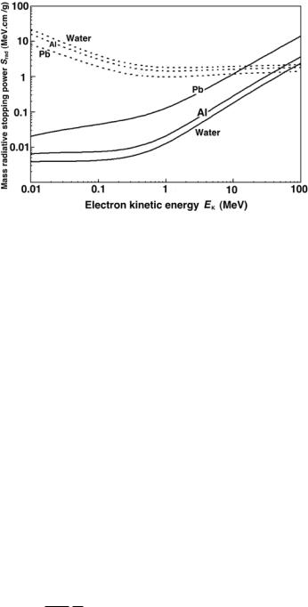
Figure 5.2 shows the mass radiative stopping power Srad for electrons in water, aluminum and lead based on tabulated data obtained from the National Institute of Standards and Technology (NIST) in Washington, D.C., USA. The Srad data are shown with solid curves, mass collision stopping powers Scol (discussed in Sect. 5.3) are shown dotted for comparison. The radiative stopping power Srad clearly shows an approximate proportionality to the atomic number Z of the absorber and kinetic energy EK of light charged particles with kinetic energies above 2 MeV.

5.3 Collision Stopping Power for Heavy Charged Particles

In the energy range below 10 MeV, the energy transfer from energetic heavy charged particles to a medium (absorber) they traverse occurs mainly through Coulomb interactions of the charged particle with orbital electrons of the absorber atoms. As shown schematically in Fig. 5.1, these interactions (collisions) fall into two categories depending on the relative magnitude of the impact parameter b and the atomic radius a of the absorber:

1.soft collisions for b a

2.hard collisions for b ≈ a

5.3 Collision Stopping Power for Heavy Charged Particles

145

Fig. 5.2. Mass radiative stopping power for electrons in water, aluminum and lead shown with solid curves against the electron kinetic energy. Mass collision stopping powers for the same materials are shown with dotted curves for comparison. Data were obtained from the NIST

5.3.1 Momentum Transfer from Heavy Charged Particle to Orbital Electron

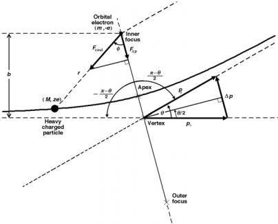
The classical derivation of the mass collision stopping power Scol of a heavy charged particle, such as a proton, is based on the calculation of the momentum change ∆p of the heavy charged particle colliding with an orbital electron. The Coulomb interaction between the heavy charged particle (charge ze and mass M ) and the orbital electron (charge e and mass me) is shown schematically in Fig. 5.3. The situation here appears similar to that depicted in Fig. 2.3 for Rutherford scattering between an α particle mα and gold nucleus M . We must note, however, that in Rutherford scattering mα M , while the case here is reversed as we have a heavy charged particle M interacting with an orbital electron me where M me.

The momentum transfer ∆p is along a line that bisects the angle π − θ, as indicated in Fig. 5.3, and the magnitude of ∆p is calculated as follows:

	∞
∆p = F∆pdt =	Fcoul cos φ dt .	(5.8)

−∞

The magnitude of the Coulomb force Fcoul between the heavy charged particle and the electron is

Fcoul =	ze2 1	,	(5.9)
	4πεo r2

where r is the distance between the two particles.

146 5 Interactions of Charged Particles with Matter

Fig. 5.3. Schematic diagram of a collision between a heavy charged particle M and an orbital electron me. Since M me, the scattering angle θ ≈ 0◦ . The scattering angle is shown larger than 0◦ to highlight the principles of the Coulomb collision and aid in the derivation of ∆p. The electron is in the inner focus of the hyperbola because of the attractive Coulomb force between the positive charged particle and the negative electron

Incorporating the expression for the Coulomb force into (5.8), the momentum transfer ∆p can now be written as

			π−θ
		ze2	2	cos φ dt
	∆p =							(5.10)
							dφ ,
		4πεo		r2		dφ

−π−θ

2

where φ is the angle between the radius vector r and the bisector, as shown in Fig. 5.3.

The angular momentum L for the collision process is defined as follows:

L = M υ	∞	b = M ωr2	,	(5.11)

where

M is the mass of the heavy charged particle,

v∞ is the initial velocity of the heavy charged particle (i.e., velocity before the interaction),

ωis the angular frequency equal to dφ/dt.

5.3 Collision Stopping Power for Heavy Charged Particles

147

Using the conservation of angular momentum, we can now write (5.10) in a simpler form:

						π−θ
		ze2 1				2		ze2 1
	∆p =						cos φ dφ =				{sin φ}−(π−θ)/2
		4πεo υ∞b						4πεo υ∞b
											(π−θ)/2

−π−θ

2

	= 2	ze2 1				cos	θ	.	(5.12)
		4πεo υ∞b					2

Equation (5.12) is identical to Rutherford’s expression for ∆p in (2.12). However, in the case of a heavy charged particle (ze) interacting with a stationary orbital electron (e) the scattering angle θ ≈ 0, and thus results in a simplified expression for ∆p since cos(θ/2) ≈ 1

∆p = 2	ze2	1		.	(5.13)
4πεo υ∞b

The energy transferred to the orbital electron from the heavy charged particle for a single interaction with an impact parameter b is

(∆p)2

e2

2

z2

∆E(b) =

= 2

,

(5.14)

2me

4πεo

meυ∞2 b2

using the classical expression between kinetic energy EK = mυ2

/2 and mo-

mentum p = mυ∞

∞

mυ2

p2

EK =

2∞

=

.

(5.15)

2m

Note that in (5.14) me is the rest mass of the electron (target) and υ∞ is the velocity of the heavy charget particle (projectile).

5.3.2 Linear Collision Stopping Power

The total energy loss of the charged particle in the absorber per unit path length dE/dx is defined as the linear stopping power. It is calculated by integrating ∆E(b) over all possible impact parameters b ranging from bmin to bmax and accounting for all electrons available for interaction to obtain

	dE			bmax		∆n
			=		∆E(b)			(5.16)
	−						.
		dx				∆x

bmin

The mass collision stopping power Scol is calculated from the linear collision stopping power with the standard relationship

Scol = −	1 dE	(5.17)
	ρ dx .

148 5 Interactions of Charged Particles with Matter

In (5.16) ∆n/∆x is the number of electrons per unit path length in a thin annual cylinder with inner radius b and outer radius b + db. The cylinder’s axis is aligned with the trajectory of the heavy charged particle.

Intuitively we may consider integration in (5.16) over all possible impact parameters from 0 to ∞; however, we must account for two physical limitations a ecting the energy transfer from a heavy charged particle to orbital electrons:

1.Minimum possible energy transfer is governed by the ionization and excitation potentials of orbital electrons resulting in a maximum impact parameter bmax beyond which energy transfer becomes impossible.

2.Maximum possible energy transfer in a head-on collision between the heavy charged particle and the orbital electron was discussed in Sect. 4.3 and results in a minimum impact parameter bmin.

The number of electrons ∆n contained in the annual cylinder with radii b and b + db is

∆n = Nedm = (ZNA/A)dm ,

(5.18)

where

Ne is the number of electrons per unit mass (ZNA/A) in the absorber,

dm is the mass contained in the annual cylinder between b and b+db equal to

dm = ρdV = ρπ(b + db)2∆x − ρπb2∆x

= ρπ∆x[b2 + 2b(db) + (db)2 − b2] ≈ 2π ρ b db ∆x .

(5.19)

Ignoring the (db)2 term in (5.19) we express ∆n/∆x as follows:

∆n/∆x = 2π ρ(ZNA/A)b db .

(5.20)

The mass collision stopping power Scol is then equal to

1 dE

e2

2

bmax

z2

db

Scol = −

= 4πNe

ρ

dx

4πεo

meυ∞2

b

bmin

= 4πNe

e2

2

z2

bmax

ln

.

(5.21)

4πεo

meυ∞2

bmin

Z

e2

2

z2

bmax

= 4π

NA

ln

.

(5.22)

A

4πεo

meυ∞2

bmin

The mass collision stopping power exhibits: (1) linear proportionality with z2, the atomic number of the heavy charged particle (projectile) and (2) inverse proportionality with υ∞2 , the initial velocity of the projectile. This implies, for example, that mass collision stopping powers of an absorbing medium will di er by: (1) factor of 4 in the case of protons and α particles of same velocities; (2) factor of 16 in the case of protons and α particles of same kinetic energies.