

Radiation Physics for Medical Physiscists - E.B. Podgorsak
.pdf8.3 Radioactive Series Decay |
269 |
The rate of change dND/dt in the number of daughter nuclei D is equal to the supply of new daughter nuclei D through the decay of P given as λPNP(t) and the loss of daughter nuclei D from the decay of D to G given as [−λDND(t)], i.e.,
dND/dt = λPNP(t) − λDND(t) = λPNP(0) e−λPt − λDND(t) ,(8.21)
where NP(0) is the initial number of parent nuclei at time t = 0.
The parent P follows a straightforward radioactive decay process with the
initial condition NP(t = 0) = NP(0), as described by (8.7) |
|
NP(t) = NP(0) e−λPt . |
(8.22) |
We are now interested in obtaining the functional relationship for the number of daughter nuclei ND(t) assuming an initial condition that at t = 0 there are no daughter nuclei D present. The initial condition for the number of daughter nuclei ND is thus as follows:
ND(t = 0) = ND(0) = 0 . |
(8.23) |
The general solution of the di erential equation given by (8.21) will be of the form
ND(t) = NP(0) |
pe−λP t + de−λD t , |
(8.24) |
where p and d are constants to be determined using the following four steps:
1. Di erentiate (8.24) with respect to time t to obtain |
|
|
dN |
−pλPe−λPt − dλDe−λDt . |
|
dtD = NP(0) |
(8.25) |
|
2. Insert (8.24) and (8.25) into (8.21) and rearrange the terms to get
e−λPt {−pλP − λP + pλD} = 0 . |
(8.26) |
3.The factor in curly brackets of (8.26) must be equal to zero to satisfy the equation for all values of t, yielding the following expression for the constant p:
p = |
λP |
(8.27) |
λD − λP . |
4.The coe cient d depends on the initial condition for ND at time t = 0, i.e., ND(t = 0) = 0 and may now be determined from (8.24) as
p + d = 0 |
|
|
(8.28) |
or after inserting (8.27) |
|
||
d = −p = − |
λP |
(8.29) |
|
|
. |
||
λD − λP |
|||


8.3 Radioactive Series Decay |
271 |
respectively, as
|
|
|
|
|
|
|
|
ln |
(t1/2)D |
|
|
|
|
|
|
|
|
|
|
|
|
|
||||||||
(tmax)D = |
|
|
|
|
|
|
|
(t1/2)P |
|
|
|
|
|
|
|
|
|
|
|
|
||||||||||
|
|
|
|
|
|
|
|
|
|
|
|
|
|
|
|
|
|
|
|
|
|
|||||||||
|
|
|
|
|
|
|
1 |
|
|
|
|
|
|
|
|
1 |
|
|
|
|
|
|
|
|
|
|||||
ln2 |
|
|
|
|
|
|
− |
|
|
|
|
|
|
|
|
|
|
|
|
|||||||||||
(t |
|
|
|
) |
|
|
(t |
|
|
|
)D |
|
|
|||||||||||||||||
|
|
|
|
|
|
|
|
1/2 |
|
P |
|
|
|
1/2 |
|
(t1/2)D |
|
|
||||||||||||
|
|
|
(t1/2)P(t1/2)D |
|
|
ln |
|
|
|
|
|
|
||||||||||||||||||
= |
|
(t1/2)P |
|
(8.35) |
||||||||||||||||||||||||||
(t1/2)D − (t1/2)P |
|
|
|
|
ln2 |
|
||||||||||||||||||||||||
and |
|
|
|
|
|
|
|
|
|
|
|
|
|
|
|
|
|
|
|
|
|
|
|
|
|
|
||||
|
|
|
|
|
τD |
|
|
|
|
|
|
|
|
τPτD |
|
|
|
|
τP |
|
|
|
||||||||
(tmax)D = |
|
ln τP |
|
|
|
= |
|
|
|
|
ln |
. |
(8.36) |
|||||||||||||||||
1 |
|
|
|
|
1 |
|
|
τP − τD |
|
|
|
|
||||||||||||||||||
|
|
|
|
|
− |
|
|
|
|
|
|
|
|
τD |
|
|
||||||||||||||
|
|
τD |
τP |
|
|
|
|
|
|
|
|
|||||||||||||||||||
8.3.3 General Form of Daughter Activity
Equations (8.33), (8.35) and (8.36) show that (tmax)D is positive and real, irrespective of the relative values of λP and λD, except for the case of λP = λD for which AD(t) in (8.31) is not defined.
At t = (tmax)D, we get from (8.31) that AP[(tmax)D] = AD[(tmax)D], i.e., the activities of the parent and daughter nuclei are equal and the condition referred to as the ideal equilibrium is met. The term ideal equilibrium was introduced by Robley Evans to distinguish this instantaneous condition from other types of equilibrium (transient and secular) that are defined below for the relationship between the parent and daughter activity under certain special conditions.
•For 0 < t < (tmax)D, the activity of parent nuclei AP(t) always exceeds the activity of the daughter nuclei AD(t), i.e., AD(t) < AP(t).
•For (tmax)D < t < ∞, the activity of the daughter nuclei AD(t) always exceeds, or is equal to, the activity of the parent nuclei AP(t), i.e., AD(t) AP(t).
Equation (8.31), describing the daughter activity AD(t), can be written in a general form covering all possible physical situations. This is achieved by introducing variables x, yP, and yD as well as a decay factor m defined as
1. x: time t normalized to half-life of parent nuclei (t1/2)P |
|
||
x = |
t |
, |
(8.37) |
(t1/2)P |
|||
2.yP: parent activity AP(t) normalized to AP(0), the parent activity at t = 0
yP = |
AP(t) |
= e−λPt |
[see (8.8) and (8.22)] , |
(8.38) |
|
AP(0) |
|
|
|

272 8 Radioactivity
3.yD: daughter activity AD(t) normalized to AP(0), the parent activity at t = 0
yD = |
AD(t) |
, |
(8.39) |
|
AP(0) |
|
|
4.m: decay factor defined as the ratio of the two decay constants, i.e.,
λP/λD
m = |
λP |
= |
(t1/2)D |
, |
(8.40) |
|
λD |
|
(t1/2)P |
||||
|
|
|
|
|
||
Insertion of x, yD, and m into (8.31) results in the following expression for yD, the daughter activity AD(t) normalized to the initial parent activity AP(0)
yD = 1 − m e− |
|
− e− |
|
|
= 1 − m |
|
2x |
− |
2 m |
. (8.41) |
||||
1 |
|
x ln 2 |
|
x |
ln 2 |
1 |
|
1 |
|
1 |
|
|
||
|
|
|
|
|
m |
|
|
|
|
|
|
x |
|
|
Equation (8.41) for yD as a function of x has physical meaning for all positive values of m except for m = 1 for which yD is not defined. However, since (8.41) gives yD = 0/0 for m = 1, we can apply the L’Hˆopital’s rule and determine the appropriate function for yD as follows:
|
|
d |
|
1 |
|
|
|
1 |
|
|
|
|
|
||
|
|
|
|
|
|
− |
|
|
|
|
|
|
|
|
|
yD(m = 1) = lim |
dm |
|
2x − |
2x/m |
|
|
|
|
|||||||
|
|
d |
|
|
|
|
|
|
|
|
|||||
m→1 |
|
|
(1 |
|
m) |
|
|
|
|
||||||
|
|
dm |
|
|
|
|
|
||||||||
|
|
|
|
x |
|
|
|
|
x |
|
|
|
|
||
|
−2− m ln 2 |
|
|
x |
|
|
|||||||||
lim |
|
|
m2 |
|
|
|
|||||||||
|
|
|
|
|
= (ln 2) |
2x . |
(8.42) |
||||||||
= m→1 |
|
|
|
|
−1 |
|
|
|
|||||||
Similarly, (8.15) for the parent activity AP(t) can be written in terms of variables x and yP as follows:
yP = e−λPt = e−x ln 2 = |
1 |
, |
(8.43) |
|
2x |
||||
|
|
|
where x was given in (8.37) as x = t/(t1/2)P and yP = AP(t)/AP(0) is the parent activity AP(t) normalized to the parent activity AP(0) at time t = 0.
The characteristic time (tmax)D can now be generalized to xmax by using
(8.37) to get the following expression: |
|
||||
(xmax)D = |
(tmax)D |
. |
(8.44) |
||
|
|||||
|
(t |
1/2 |
) |
|
|
|
|
P |
|
||
Three di erent approaches can now be used to determine (xmax)D for yD in (8.41)
1. Set (dyD/dx) = 0 at x = (xmax)D and solve for (xmax)D to get |
(8.45) |
|||||||||||||||
|
dx x=xmax = 1 |
|
|
|
m −2−x + m 2− m x=xmax = 0 . |
|||||||||||
|
dyD |
|
|
|
ln 2 |
1 |
|
x |
|
|
||||||
|
|
|
|
− |
|
|
|
|
|
|
|
|
||||
|
|
|
max |
D |
|
we finally get |
|
|
|
|||||||
Solving (8.45) for (x |
) |
|
|
|
|
|
|
|||||||||
(xmax)D = |
m |
|
|
|
log m |
= |
m ln m |
. |
|
(8.46) |
||||||
|
|
|
|
|
|
|
||||||||||
m − 1 |
log 2 |
m − 1 |
ln 2 |
|
||||||||||||

8.3 Radioactive Series Decay |
273 |
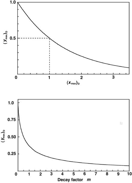
Fig. 8.2. Variable yD of (8.41) against variable x for various values of decay parameter m. The dashed curve is for yP of (8.43) against x. The parameter (xmax)D shown by dots on the yP curve is calculated from (8.46). Values for (yD)max are obtained with (8.49)
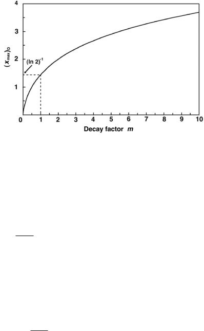
For m = 1 (8.46) is not defined; however, since it gives xmax = 0/0, we can apply the L’Hopital’s rule to get (xmax)D|m→1 as follows:
|
|
|
|
|
|
d(m ln m) |
|
|
|
|
|
|
|
||
(x |
max)D|m→1 |
lim |
|
|
dm |
|
|
|
|
|
|
|
|||
|
|
d(m−1) |
|
|
|
|
|||||||||
|
= m |
→ |
1 |
ln 2 |
|
|
|
|
|||||||
|
|
|
|
dm |
|
|
|
|
|
|
|
||||
|
|
= lim |
1 + ln m |
|
= |
1 |
|
= 1.44 , |
(8.47) |
||||||
|
|
|
ln 2 |
ln 2 |
|||||||||||
|
|
m→1 |
|
|
|
|
|
|
|||||||
Thus, (xmax)D is calculated from (8.46) for any positive m except for m = 1. For m = 1, (8.47) gives xmax = 1.44.
2.Insert (8.37) and (8.40) into (8.33) for (tmax)D and solve for (xmax)D to get the result given in (8.46).
3.Recognize that when x = (xmax)D the condition of ideal equilibrium applies for (8.41), i.e., yP[(xmax)D] = yD[(xmax)D]. Insert x = (xmax)D into (8.41) and (8.43), set yP[(xmax)D] = yD[(xmax)D], and solve for (xmax)D to get the result of (8.46).
In Fig. 8.2 we plot (8.41) for yD against x using various values of the decay factor m in the range from 0.1 to 10.0. For comparison we also plot yP of (8.43) against x (dotted curve).
The function plotted as a dashed curve for m = 1 in Fig. 8.2 is the function given in (8.42). The point of ideal equilibrium for this curve occurs at xmax given as (1/ ln 2) = 1.44 in (8.47) and at yD(xmax) = 1/e = 0.368.
274 8 Radioactivity
All yD curves of Fig. 8.2 start at the origin at (0,0), rise with x, reach a peak at (xmax)D, as given in (8.46), and then decay with an increasing x. The smaller is m, the steeper is the initial rise of yD, i.e., the larger is the initial slope of yD. The initial slope and its dependence on m can be determined from the derivative dyP/dx of (8.45) by setting x = 0 to get
dx |
x=0 = |
1 m |
−2−x + m |
2− m x=0 = |
m . |
(8.48) |
||||
dyD |
ln 2 |
1 |
|
x |
|
ln 2 |
|
|||
|
|
− |
|
|
|
|
|
|
|
|
|
|
|
|
|
|
|
|
|
|
|
|
|
|
|
|
|
|
|
|
|
|
Noting that x = t/(t1/2)P, m = λP/λD, and yD = AD(t)/AP(0), we can link the data of Fig. 8.2 with physical situations that occur in nature in the range
0.1 < m < 10. Of course, the m region can be expanded easily to smaller and larger values outside the range shown in Fig. 8.2 as long as a di erent scale for the variable x is used.
As indicated with dots on the yP curve in Fig. 8.2, (ymax)D, the maxima in yD for a given m, occur at points (xmax)D where the yD curves cross over the yP curve. The xmax values for a given m can be calculated from (8.46) and (yD)max for a given m can be calculated simply by determining yP(x) at x = xmax with yP(x) given in (8.43). We thus obtain the following expression for (ymax)D:
(y ) = y (x |
) = 2( 1−m ) ln 2 |
= |
1 |
|
e 1−m ln m |
|||
|
|
m ln m |
|
≡ |
|
m |
||
max D P |
max D |
|
|
|
|
|
||
|
2(xmax)D |
|
|
|
||||
= e−(ln 2)(xmax)D , |
|
|
|
(8.49) |
||||
where (xmax)D was given by (8.46). Equation (8.49) is valid for all positive m with the exception of m = 1. We determine (yD)max for m = 1 by applying the L’Hˆopital’s rule to (8.49) to get
|
|
|
|
|
|
d |
|
|
(m ln m) |
|
|
|
|
||
(y |
|
|
|
|
|
dm |
ln m+1 |
1 |
|
||||||
|
|
|
|
|
|
|
|
||||||||
|
|
|
|
|
d |
|
|
|
|
|
|||||
) |
D|m=1 |
= lim 2 |
|
|
|
(1−m) ln 2 |
= lim 2 − ln 2 |
= 2− |
ln 2 |
|
|||||
dm |
|||||||||||||||
|
max |
m→1 |
|
|
|
|
m→1 |
|
|
|
|||||
|
|
|
= e−1 = 0.368 . |
|
(8.50) |
||||||||||
As shown in (8.49), (ymax)D and (xmax)D are related through a simple exponential expression plotted in Fig. 8.3 and also given by (8.43) with x = (xmax)D and yP = (ymax)D. As shown in (8.49) the ideal equilibrium value (ymax)D exhibits an exponential decay behavior starting at (ymax)D = 1 at (xmax)D = 0 through (ymax)D = 0.5 at (xmax)D = 1 to approach 0 at
(xmax)D → ∞.
Figures 8.4 and 8.5 show plots of (ymax)D and (xmax)D, respectively, against m as given by (8.49) and (8.46), respectively, for positive m except for m = 1. The m = 1 values of (xmax)D and (ymax)D, equal to 1/ ln 2 and 1/e, respectively, were calculated from (8.47) and (8.50), respectively. With increasing m, the parameter (xmax)D starts at zero for m = 0, goes through 1/ ln 2 = 1.44 at m = 1, and then increases as ln m for very large m. Parameter (ymax)D, on the other hand, starts at 1 for m = 0, goes through 1/e = 0.368 at m = 1, and then decreases exponentially for very large m.
278 8 Radioactivity
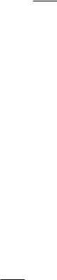
2.For the 0 < m < 1 region, (8.54) suggests that the exponential term diminishes with increasing x and exponentially approaches zero. This means that at large x the parameter ξ approaches a constant value that is independent of x and is equal to 1/(1 − m). Under these conditions the parent activity AP(t) and daughter activity AD(t) are said to be in transient equilibrium, and are governed by the following relationship:
ξ = |
AD(t) |
= |
yD |
= |
1 |
= |
|
1 |
= |
λD |
|
. (8.57) |
|
|
|
|
|
− λP/λD |
λD − |
|
|||||||
|
AP(t) |
|
yP |
1 − m 1 |
|
λP |
|||||||
After initially increasing, the daughter activity AD(t) goes through a maximum and then decreases at the same rate as the parent activity AP(t) and the two activities are related through (8.57). As m decreases, the daughter and parent activities at relatively large times t become increasingly more similar, since, as m → 0, ξ → 1. This represents a special case of transient equilibrium (λD λP, i.e., m → 0) and in this case the parent and daughter are said to be in secular equilibrium. Since in secular equilibrium ξ = 1, the parent and daughter activities are approximately equal, i.e., AP(t) ≈ AD(t) and the daughter decays with the same rate as the parent.
Equations (8.51) and (8.54) are valid in general, irrespective of the relative magnitudes of λP and λD; however, as indicated above, the ratio AD(t)/AP(t) falls into four distinct categories that are clearly defined by the relative magnitudes of λP and λD. The four categories are:
(1) Daughter Longer-Lived Than Parent:
(t1/2)D > (t1/2)P, i.e., λD < λP.
We write the ratio AD(t)/AP(t) of (8.51) as follows:
AP(t) |
λP − λD |
|
− |
|
|
|
AD(t) |
= |
λD |
e(λP−λD)t |
|
1 . |
(8.58) |
|
|
|||||
No equilibrium between the parent activity AP(t) and the daughter activity AD(t) will be reached for any t.
(2) Half-Lives of Parent and Daughter are Equal:
(t1/2)D = (t1/2)P, i.e., λD = λP.
The condition is mainly of theoretical interest as no such example has been observed in nature yet. The ratio AD(t)/AP(t) is given as a linear function, as shown in (8.55).