The Physics of Coronory Blood Flow - M. Zamir

5.2 Basic Theory

149

where the A’s and B’s are constants known as “Fourier coe cients” and are given by

		1		0	T
	A0 =				p(t)dt					(5.2.15)
		T
		2			T		2nπt		dt
	An =			0	p(t) cos					(5.2.16)
		T					T
		2			T	2nπt
	Bn =			0	p(t) sin				dt	(5.2.17)
		T					T

The infinite series in Eqs.5.2.13,14 are called Fourier series, and this representation of the function p(t) is then referred to as the Fourier series representation of that function.

We note from the definition of A0 that it represents the average value of the periodic function p(t) over one period. We note further that there are actually two series in Eq. 5.2.14 and that, except for A0, the remaining terms in the two series are paired, meaning that the terms in A1 and B1 have the same argument, namely 2πt/T , and the next two terms again have the same argument, namely 4πt/T , etc. This makes it possible to combine each pair, using standard trigonometric identities, whereby we can write

A1 cos	T		+ B1 sin		T	= M1 cos		2 T	− φ1		(5.2.18)
	2nπt				2nπt			nπt
where M1, φ1 are two new constants, related to A1, B1 by
			A1	= M1 cos φ1							(5.2.19)
			B1	= M1 sin φ1							(5.2.20)

This pairing process can now be repeated for each pair of terms in Eq. 5.2.14, with the result that the two Fourier series can be combined into one, namely

p(t) = A0	+ M1 cos		2T	− φ1	+ M2 cos	T − φ2
			πt			4πt

+M3 cos	6πt		+ ...			(5.2.21)
		− φ3
	T
or in more compact form
p(t) = A0	+ n=1 Mn cos			2 T − φn		(5.2.22)
	∞			nπt

where

150	5 The Analysis of Composite Waveforms
	An = Mn cos φn	(5.2.23)
	Bn = Mn sin φn	(5.2.24)

Eq. 5.2.22 provides a more compact Fourier series representation of the function p(t) because it contains only one series instead of two. In this representation each term except the first is a simple cosine wave with M as its amplitude and φ as its phase. Because these waves add up to constitute the function p(t), they are referred to as the “harmonics” of this periodic function.

We note in Eq. 5.2.22 that in the first harmonic the cosine function has the same value at t = 0 and at t = T , therefore this harmonic has a period T , which is the same as the period of the original function p(t). For this reason it is referred to as the “fundamental harmonic”. In the second harmonic, by comparison, the cosine function has the same value at t = 0 and at t = T /2. Therefore, this harmonic has a period T /2 which is half the period of p(t). This pattern continues to higher harmonics.

Because of the reciprocal relation between the period and the frequency of a periodic function, the above pattern can be expressed in terms of the frequencies of the harmonics. Thus, if f is the frequency of the periodic function p(t) in cycles per second (Hz), then

				f =	1		(5.2.25)
					T
	and the angular frequency ω is given by
	ω = 2πf						(5.2.26)
	=	2π		radians per second			(5.2.27)
		T

Thus the Fourier series representation in Eq. 5.2.22 can now be put in the

form
p(t) = A0 + M1 cos (ωt − φ1) + M2 cos (2ωt − φ2)
+M3 cos (3ωt − φ3) + ...	(5.2.28)

in which it is seen clearly that the frequency of the first harmonic is ω, the same as the frequency of the original function p(t) and is therefore referred to as the “fundamental frequency”. The frequency of the second harmonic is 2ω, and of the third is 3ω, etc. These are important properties of the harmonics of a periodic function which we shall see more clearly later as we consider specific functions. In particular, we shall see that in many cases the first 10 harmonics are su cient for producing a good representation of a given periodic function such as the composite pressure wave produced by the heart. In that case, the fundamental frequency is the beating frequency of the heart which, under resting conditions, is approximately 1 Hz, thus the frequency of the tenth harmonic would be 10 Hz. It is for this reason that frequencies as high as 10 Hz are considered in the dynamics of the coronary circulation and of the cardiovascular system in general.

5.3 Example: Single-Step Waveform

151

5.3 Example: Single-Step Waveform

The theory of Fourier analysis described in the previous section is well established and fairly straightforward, but its application to the analysis of specific composite waveforms involves some tedious calculations and some algebraic intricacies which can only be illustrated by considering a specific example. While mathematical software packages now have specific tools under the heading of Fast Fourier Transforms (FFT) that can handle much of the tedious calculations, these tools cannot be used reliably without a basic understanding of the analytical intricacies involved [28, 197]. For this reason, in this and subsequent sections we consider a series of examples that are intended to illustrate the analytical process involved, starting with a very simple example in this section. In each case, the purpose of the analysis is to find the Fourier series representation of the given waveform, that is to find the series of sine and cosine waves of which the given waveform consists.

Consider the simple waveform consisting of a single step shown in Fig. 5.3.1, which has a period T = 1 as seen graphically, and which is defined by the function

p(t) = 1,	0 ≤ t <			1		(5.3.1)
				2
= 0,	1		≤ t < 1			(5.3.2)
		2

Following the theory presented in the previous section, the Fourier series representation of this periodic function is given by (Eq. 5.2.13)

∞

nπt

∞

2nπt

(5.3.3)

p(t) = n=0 An cos

2 T

+ n=1 Bn sin

T

= A0 + A1 cos

2T

+ A2 cos

T

+ ...

πt

4πt

4T

+B1 sin

T

+ B2 sin

+ ...

(5.3.4)

2πt

πt

and, using Eqs.5.2.15-17 to find the Fourier coe cients, recalling that T = 1 in this case, we have

		1		T
A0 =				0	p(t)dt		(5.3.5)
		T
=	0			1 p(t)dt			(5.3.6)
=	1/2				1 × dt + 1	0 × dt	(5.3.7)

01/2

	=	1	(5.3.8)
		2

152 5 The Analysis of Composite Waveforms

1.5
1
0.5
0
−0.5	0.5	1
0
4

2

0
−2	1	2	3	4
0

Fig. 5.3.1. A simple waveform consisting of a single step and having a period T = 1 as seen in the left two panels. The first ten harmonics of this waveform are shown on the right. The even harmonics, namely harmonics 2, 4, 6, 8, 10 are zero in this case and make no contribution to the Fourier composition of this waveform, as seen on the right. The series is led by the fundamental harmonic which has the same period and hence the same frequency as the original wave, namely the fundamental period and fundamental frequency. The period of the third harmonic is one third of the fundamental period and hence its frequency is three times the fundamental frequency, etc.

Note that by its definition (Eq. 5.3.5), A0 represents the average value of the periodic function over one period, which in Fig. 5.3.1 is seen graphically to be 1/2, in agreement with the above result.

	2				T	p(t) cos	2nπt	dt
An =				0							(5.3.9)
		T					T
=	2		0		1 p(t) cos(2nπt)dt						(5.3.10)
			0		1/2				1
=	2					1 × cos(2nπt)dt + 2			1/2	0 × cos(2nπt)dt	(5.3.11)
=	2				1/2 cos(2nπt)dt						(5.3.12)

0

5.3

Example: Single-Step Waveform

153

sin(2nπt)

1/2

=

nπ

0

(5.3.13)

= 0

for all n

(5.3.14)

2

T

2nπt

Bn =

0

p(t) sin

dt

(5.3.15)

T

T

= 2

0

1 p(t) sin(2nπt)dt

(5.3.16)

0

1/2

1

= 2

1 × sin(2nπt)dt + 2

1/2

0 × sin(2nπt)dt

(5.3.17)

= 2

0

1/2 sin(2nπt)dt

(5.3.18)

cos(2nπt)

1/2

=

−

nπ

0

(5.3.19)

1

cos nπ

=

−

nπ

(5.3.20)

Substituting these values of the Fourier coe cients in Eqs.5.3.4, we obtain

the required Fourier series representation of this waveform, namely

p(t) =

1

∞

1

cos nπ

(5.3.21)

2

+ n=1

− nπ

sin (2nπ)

=

1

+

2

sin (2nπ) + 0 +

2

sin (6nπ) + 0 . . .

2

2

π

3π

+

sin (10nπ) + 0 . . .

(5.3.22)

5π

1

2

2

2

=

+

sin (2nπ) +

sin (6nπ) +

sin (10nπ) . . . (5.3.23)

2

3π

5π

π

To put the series in the more compact form of Eq. 5.2.22, that is, in terms of the amplitudes Mn and phase angles φn of the individual harmonics that

make up the waveform, we use Eqs.5.2.23,24 to find

=

(5.3.24)

M

n

A2

+ B2

n

n

= B

since An = 0 for all n

(5.3.25)

n

1

cos nπ

=

−

(5.3.26)

nπ

and

φn = tan−1

Bn

(5.3.27)

An

= ±

π

since An = 0 for all n

(5.3.28)

2

154 5 The Analysis of Composite Waveforms

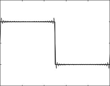
Fig. 5.3.2. Fourier series representations of the single-step waveform, based on the first one, four, seven, and ten harmonics, clockwise from top left corner.

Which of the two values of φ is appropriate is determined by satisfying Eq. 5.2.24, namely

Bn = Mn sin φn

(5.3.29)

Since Mn = Bn in this case (Eq. 5.3.25), this gives sin φn = 1, and therefore

φn =	π	for all n	(5.3.30)
	2

Substituting these values of Mn, φn into Eq. 5.2.22 gives

			∞
p(t) = A0 +				Mn cos (2nπt − φn)					(5.3.31)
			n=0
1			∞		1 cos nπ	π
					−	cos (2nπt −
=	2		+ n=0		nπ		2	)	(5.3.32)
1			∞		cos nπ
=					1 −	sin (2nπt)
	2		+ n=0		nπ				(5.3.33)

=	1	+	2	sin (2πt) +	2	sin (6πt) +	2	sin (10πt) . . . (5.3.34)
	2				3π		5π
			π

5.3 Example: Single-Step Waveform

155

	1.5
	1
magnitude	0.5
	0
	−0.50	0.2	0.4	0.6	0.8	1
				time

Fig. 5.3.3. Fourier series representation of the single-step waveform based on the first 50 harmonics.

which is identical with the result in Eq. 5.3.23.

Thus, in the present example, because of the very simple form of the wave, the two di erent forms of Fourier series representation in Eqs.5.2.13,22 are identical. More precisely, the Fourier series representation of this simple waveform consists of only one series (not two as in Eq. 5.2.13), hence the compact and the non-compact forms of the Fourier represenation are the same. Furthermore, we shall find that the determination of the phase angle φ is in general more troublesome than it is in the present simple case. The reason for this is that the range of the inverse tangent function used in Eq. 5.3.27 is limited to the interval −π/2 to +π/2 and therefore does not yield all possible angles.

If the harmonics of this waveform are denoted by p1(t), p2(t), p3(t) . . ., then

the result in Eq. 5.3.34 can be written as
p(t) =	1
			+ p1(t) + p2(t) + p3(t) . . .				(5.3.35)
		2
where the individual harmonics are given by
		p1		(t) =	2	sin (2πt)	(5.3.36)
					π
		p2		(t) = 0			(5.3.37)

156 5 The Analysis of Composite Waveforms

p3	(t) =	2	sin (6πt)	(5.3.38)
		3π
p4	(t) = 0			(5.3.39)
	.
	.
	.

It is seen that the first harmonic has the same period and hence the same frequency as the original wave, namely the fundamental period and fundamental frequency. The second and other even-numbered harmonics are zero in this case. The period of the third harmonic is one third of the fundamental period and hence its frequency is three times the fundamental frequency, etc. The first ten harmonics are shown graphically in Fig. 5.3.1.

magnitude

1.5

1

0.5

0

−0.50	0.2	0.4	0.6	0.8	1
			time

Fig. 5.3.4. Fourier series representation (circles) of the single-step waveform (solid line) based on a Fast Fourier Transform (FFT) program. Such programs, which are available with most mathematical software packages, use an appropriate number of harmonics to produce highly accurate Fourier series representations.

One of the most important pillars of the theory of Fourier analysis is that the amplitudes of successive harmonics become successively smaller and hence they make successively smaller contribution to the Fourier representation of the periodic function in hand. This is highly important for practical purposes because the infinite series representing the periodic function can then be truncated at some point without committing large error. This is illustrated graph-

5.4 Example: Piecewise Waveform

157

ically in Fig. 5.3.2, where di erent Fourier series representations are shown, based on the first one, four, seven, and ten harmonics. A Fourier series representation based on the first 50 harmonics is shown in Fig. 5.3.3 where these properties can be observed. We shall see later that a larger number of harmonics does not always produce a more accurate Fourier series representation. Specifically, when the description of a given periodic function is available in only numerical form, as in Table 5.1.1 for the cardiac wave, new complications arise which make the optimum number of harmonics dependent on the number of data points available in the numerical description of the waveform.

Computer programs based on the Fast Fourier Transform (FFT) are optimized to use a number of harmonics appropriate for the number of data points available [28, 197], to produce a highly accurate Fourier series representation of a given periodic function, as illustrated in Fig. 5.3.4.

5.4 Example: Piecewise Waveform

Consider next a composite waveform consisting of several steps, as shown in Fig. 5.4.1, and defined by the function

p(t) =	4t,				0 ≤ t <			1					(5.4.1)
									4
=	1,			1			≤ t <	1					(5.4.2)
				4				2
=	1		,	1			≤ t <	3					(5.4.3)
		2			2					4
=	0,			3			≤ t < 1						(5.4.4)
				4

Following the theory presented in the Section 5.2, the Fourier series representation of this periodic function is given by (Eq. 5.2.13)

∞

nπt

∞

2nπt

(5.4.5)

p(t) = n=0 An cos

2 T

+ n=1 Bn sin

T

= A0 + A1 cos

2T

+ A2 cos

T

+ ...

πt

4πt

4T

+B1 sin

T

+ B2 sin

+ ...

(5.4.6)

2πt

πt

and, using Eqs. 5.2.15–17 to find the Fourier coe cients, recalling that T = 1 in this case, we have

		1	0	T
	A0 =			p(t)dt	(5.4.7)
		T

158 5 The Analysis of Composite Waveforms

1.5
1
0.5
0
−0.5		0.5		1
0
4
2
0
−2	1	2	3	4
0

Fig. 5.4.1. A composite “piecewise” waveform consisting of several steps and having a period T = 1 as seen in the left two panels. The first ten harmonics of this waveform are shown on the right. The series is led by the fundamental harmonic which has the same period and hence the same frequency as the original wave, namely the fundamental period and fundamental frequency. The periods of the second and third harmonics are one half and one third of the fundamental period, respectively, and hence their frequencies are two and three times the fundamental frequency, etc.

= 0			1 p(t)dt														3/4 1			(5.4.8)
= 0			1/4									1/2							1
						4t × dt +					1/4					1 × dt + 1/2			× dt + 3/4	0 × dt (5.4.9)
																		2
= 2t2					1/4				1/2		+	1				3/4	+ 0			(5.4.10)
					0			+ t|1/4					2 t 1/2
	1				1				1
=			+				+													(5.4.11)
	8					4			8
=	1																			(5.4.12)
	2

Again, we note that by its definition (Eq. 5.4.7), the constant A0 represents the average value of the periodic function over one period. The result is seen to be correct from the graphical representation of the waveform in Fig. 5.4.1. For the other Fourier coe cients we have

			2		T	2nπt	dt
	An =			0	p(t) cos			(5.4.13)
		T				T