Neutron Scattering in Biology - Fitter Gutberlet and Katsaras

142 J.K. Krueger et al.

minimized ( 1 mm) and they are calibrated against primary standards for a given instrument to take advantage of the intrinsically high signal-to-noise ratio for light-water samples [9, 55, 56]. However, even with the higher crosssection of water or protonated biopolymers, such isotropic scatterers cannot be used at low Q values (long sample-detector distances, r) as the intensity falls as (1/r2), and standardization requires a measurement at a low sampledetector distance, followed by scaling to the r-value of the measurement via the inverse square law [23].

The spatial variation of the detector e ciency ( ) is measured via an incoherent scatterer such as water or a protonated polymer (e.g., polymethylmethacrylate) and despite the fact that multiple scattering in such materials is not fully understood, the data are independent of angle to a good approximation [23, 40]. Thus, the variation in the measured signal is proportional to the detector e ciency, and may be used in the data analysis software to correct for this e ect on a cell-by-cell basis. Second-order corrections representing departures from isotropic scattering and unequal path lengths through di erent regions of the active gas are usually wavelength-dependent, instrumentdependent and, even detector-dependent, and Lindner and co-workers have discussed how such adjustments may be customized for a particular facility [58].

Extraction of structural information on individual macromolecules or macromolecular complexes in solution from scattering data requires samples that are rigorously aggregation free. The zero angle or forward scattering, I(0), is directly proportional to the molecular weight squared of the scattering particle and hence is extremely sensitive to aggregation [57]. For X-ray experiments, most proteins in aqueous solution have essentially the same contrast. Therefore, by using a standard protein of known concentration that is also known to be monodisperse in solution, its I(0) can be used to calculate very precise concentration values. Alternatively, if the concentrations are known, the I(0) of the standard can be used to check for sample aggregation. The relationship used for these types of analyzes, for proteins of molecular weight MX and in solution at a concentration cX, given in milligrams/milliliter, is:

I(0)X/MXcX = I(0)STD/MSTDcSTD.

(8.7)

For neutron scattering experiments, the best method for determining that samples are not aggregated is by comparing the measured I(0) values at the each of the contrasts with the expected I(0) values based on the calculated contrasts and this is only possible if the I(0) values have been put on an absolute scale using an appropriate calibration standard [23, 57].

8.3.3 Instrumental Resolution

Experimentally measured scattering data di er from the actual (theoretical) cross-sections because of departures from point geometry in a real instrument [62–66]. In general, instrumental resolution e ects are smaller for SANS

8 SANS from Biological Molecules

143

than for SAXS. This is because most SANS experiments are performed in point geometry whereas a significant proportion of X-ray experiments have used long slit sources (e.g., Kratky cameras), where smearing e ects are larger, particularly at small angles [67,68]. Less attention has been paid to resolution e ects in SANS experiments, largely because the corrections are in general smaller for point geometry. However, the corrections are not always negligible, particularly for sharply varying scattering patterns and large scattering dimensions.

In a pinhole SANS instrument (Fig. 8.4), there are essentially three contributions to the smearing of an ideal curve: (i) the finite angular divergence of the beam, ∆θ/θ = ∆φ/φ, (ii) the finite resolution of the detector, R(Q) and (iii) the polychromatic nature of the beam, ∆λ/λ. As mentioned above, for all systems discussed in this chapter, the scattering is azimuthally symmetric about the incident beam, i.e., dΣ/dΩ(Q) is a function only of the magnitude of the scattering vector |Q| = 4πλ−1 sin θ. In this case, once the instrumental parameters are well characterized, it is possible by numerical techniques not only to smear a given ideal scattering curve, but also to desmear an observed pattern by means of an indirect Fourier transform to obtain the actual Q dependence [62–66].

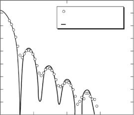
A dramatic example of smearing e ects is illustrated by SANS data from Kilham rat virus (KRV), which has a core–shell structure, and was modeled by a hollow-shell form factor [65, 69]. KRV may be prepared either “empty” or “full” of nucleic acid and a scattering from the former is shown in Fig. 8.5, which compares the actual measured scattering pattern in a pinhole SANS instrument with the simulated curve in the absence of instrumental resolution

In (I)

4.5

4.0	Experiment smeard by
	instrumental resolution
3.5	Desmeared SANS pattern

3.0

2.5

2.0

1.5

1.0

0.5

0

0	0.05	0.1	0.15	0.2
		Q (Å−1)

Fig. 8.5. Smeared and desmeared SANS data from KRV empty capsids in D2O

144 J.K. Krueger et al.

e ects using IFT methods [69]. Although SANS data are routinely analyzed without reference to smearing e ects, it is clear from Fig. 8.5 that this omission can sometimes lead to gross errors.

Another model system which has sharp features and is ideal for investigating instrumental resolution e ects is monodisperse protonated poly(methyl methacrylate) (PMMA-H) latex particles, suspended in an H2O–D2O solvent [67, 70, 71]. The scattering from a homogeneous sphere is a Bessel function [72], with sharp maxima and minima which are averaged by instrumental smearing e ects to produce a smoothly varying curve. Desmearing via IFT methods, using an algorithm due to Moore [63], leads to a sharply varying desmeared curve and a particle diameter calculated from the positions of the maxima and minima of D = 990 ˚A. This may be compared with a value of D = 992 ˚A calculated from the particle radius of gyration (Rg = 384 ˚A) derived from the desmearing procedure. The desmearing algorithm [63] used a set of transformed size functions whereas Glatter [64,66] has employed a set of cubic splines. The latter procedure leads to D = 988 ˚A [73] and thus both routines give dimensions and extrapolated Q = 0 intensities which agree within 1%. These data have also been analyzed via an algorithm employing analytical expressions for the wavelength and angular smearing in a pinhole SANS camera [74]. This simplification allows a rapid on-line least-squares desmearing analysis to be performed which leads to D = 996 ˚A, in good agreement with the above determinations. Similar agreement has been achieved for hollow (core–shell) polymer latex scattering [70, 71]. As mentioned in Section 8.3.2, IFT methods also give rise to a length distribution function, P (r), which represents the frequency of vectors connecting volume elements within the scattering particle and goes to zero at a value corresponding to the maximum dimension of the particle. P (r) is more readily interpreted in terms of structural information than the scattering profile and is sensitive to the overall shape and to the relationships between domains or repeating structures.

Where the assumption of azimuthal symmetry cannot be made, the above smearing and desmearing procedures are not applicable, and alternative procedures based on Monte Carlo (MC) techniques have been developed, which simulate the experimental smearing of a given theoretical scattering pattern that can be expressed analytically or numerically [62]. This procedure permits the estimation of resolution e ects even in anisotropic systems, but cannot facilitate the desmearing of the observed pattern. Taken together, MC and IFT methods permit a realistic evaluation of the circumstances where resolution e ects warrant correction. Both procedures have been illustrated via a range of results of experiments performed on a typical pinhole SANS facility [62], where it was shown that for experiments with scattering dimensions <200 ˚A smearing e ects are small (<5%) and that dimensions up to1000 ˚A may be resolved after proper evaluation of resolution e ects. Smearing e ects may be reduced by decreasing the wavelength range (∆λ/λ) or the angular spread (∆θ/θ), though the measured intensity is a strong function

8 SANS from Biological Molecules

145

of the resolution and Schelten has pointed out that a reduction of a factor of two in ∆Q/Q will reduce the scattered intensity by over three orders of magnitude [33].

8.3.4 Other Experimental Considerations and Potential Artifacts

For sample containment, there are several materials (e.g., quartz, singlecrystal Si), which have very little absorption or scattering for neutrons. For SAXS on the other hand, materials which have high absorption (to define a SAXS beam) also have high scattering power, as both parameters are a strong function of the atomic number, and parasitic scattering is usually higher for SAXS. Thus, the high penetrating power of neutrons makes it relatively easy to contain samples with a minimum of instrumental backgrounds.

For singly scattered neutrons, the intensity I(Q) is proportional to the sample thickness (t) and transmission (T = e− t) and is maximized for t = 1, where is the linear attenuation coe cient. Thus, the optimum sample thickness is 1–2 mm for H2O and 1 cm for D2O. Measurements in the intermediate-angle scattering range ( 0.1 < Q < 0.6 ˚A−1) are particularly sensitive to the incoherent background, which can be of the same order of magnitude as the coherent signal. This is because the coherent scattering falls rapidly with angle (e.g., as Q−2 for Gaussian coils or as Q−4 in the Porod regime [23]). The coherent intensity of singly scattered neutrons, I(Q) is proportional (Eq. 8.6) to the sample thickness (t), transmission (T ) and sample area (A). Thus, measurements on samples with di erent dimensions (t, A) and transmission (T ) may be normalized to the same volume to give a (coherent) cross-section which is an intensive (material) property, independent of the sample dimensions. This is based on the assumption that neutrons are scattered only once before being detected and this has been shown to be a reasonable approximation for coherent SANS from polymeric [77] and other materials [76], with cross-sections dΣ/dΩ(0) typically <103 cm−1, which includes most biological materials. For samples with higher cross-sections that exhibit substantial coherent–coherent multiple scattering, a common way to recognize and minimize this artifact is to measure the cross-section as a function of the sample thickness and to extrapolate to t = 0.

For incoherent scattering, 1–2 mm samples containing hydrogen (H2O, protonated polymers, etc.) give rise to appreciable multiple scattering [22,23]. The di culties in estimating an incoherent background to subtract from a given “sample” and thus isolate the residual coherent cross-section are illustrated in [77] where the apparent cross-section produced of protonated PMMA-H blanks, after normalizing via Eq. 8.6 was shown to vary by >50% over a typical range ( 0.2–1.2 mm) of sample thicknesses. Similarly, the scattering of light water contains appreciable multiple scattering [22, 23, 55, 56, 58–61], which is not proportional to the thickness or transmission, and cannot be normalized to a true cross-section which is independent of the sample dimensions. Moreover, as explained above, the bound-atom cross-section cannot

146 J.K. Krueger et al.

be used to calculate the background, because the hydrogen incoherent crosssection (σinc = 79.7 × 10−24 cm2), although widely quoted in the literature, almost never applies to real biological or aqueous-based systems. However, the incoherent scattering is independent of Q to a good approximation, and empirical methods have been developed to subtract this background [24].

8.3.5 Data Analysis: Extracting Structural and Shape Parameters from SANS Data and P (r) Analysis

Several comprehensive reviews and books have been published describing the application of SAS to biological systems [66, 78, 79] and current examples are given in this volume (e.g., see contribution by S. Krueger et al.). In combination with advances in molecular biology techniques that facilitate production of large amounts of pure protein using bacterial expression systems, substantial improvements in neutron sources and instrumentation [35–37] have broadened the impact of SAS in modern structural molecular biology. The absolute cross-section is proportional to the scattered intensity Eq. 8.6 and an initial analysis of the data may be performed to determine the scattering molecule’s Rg, along with values of the forward cross-section dΣ/dΩ(0), in a model-independent way [51] via the Guinier approximation:

dΣ/dΩ(Q) = dΣ/dΩ(0)e−Q2Rg2/3.

(8.8)

A plot of ln dΣ/dΩ(Q) versus Q2 gives a straight line with a slope of −Rg2/3 and an extrapolated intercept ln dΣ/dΩ(Q) in the region where QRg ≤ 1 (the precise upper limit of QRg for which the Guinier approximation is valid is dependent on particle shape).

For a dilute solution of monodisperse, identical particles the scattered intensity I(Q) (which is proportional to the absolute cross-section dΣ/dΩ)(Q) is related to the distribution of interatomic distances P (r) in the scattering particle by a Fourier transformation:

I(Q) = 4π P (r)[sin (Qr)/Qr]dr.

(8.9)

Eq. 8.9 assumes that the electron density of the particle is homogeneous which means that P (r) is a continuous function of r. The sin (Qr)/Qr term comes from a spatial average of all particle orientations and assumes that they are random. The inverse relationship of Eq. 8.9:

		r2
	P (r) =			I(Q)Q2[sin (Qr)/Qr]dQ,	(8.10)
		2π2
can be	used to derive the P (r) function from the experimental scattering
profile.	Several algorithms exist for calculating the P (r) from the scattering

8 SANS from Biological Molecules

147

cross-section or intensity [63,64,80], that have also been used to model instrumental resolution e ects (see above).

P (r) gives a real-space representation of the structure and thus, is more readily interpreted in terms of structural information than the scattering profile, dΣ/dΩ(Q). P (r) is sensitive to the overall shape of the scattering particle and to the relationships between domains or repeating structures. Several specific pieces of structural information can be extracted from the P (r) analysis:

(i) The P (r) goes to zero at a value corresponding to the maximum dimension of the particle, Dmax. (ii) The zeroth moment of P (r) gives the forward or zero-angle scattering, I(0), which as mentioned earlier, is proportional to the square of the molecular weight of the scattering particle. I(0) is therefore a very sensitive test for monodispersity in a protein solution of known concentration. Alternatively, it can be a sensitive indicator of macromolecular association and polymerization. Additionally, (iii) a value for Rg can be calculated using the entire angular range of the scattering profile by calculating the second moment of the P (r) distribution Eq. 8.11.

Rg2 =	P (r)r2d3	r		P (r)d3r.	(8.11)
		2

Shape information in the form of electron (or nuclear) density distribution is contained within all SAS data. Extraction of that shape information has become more and more sophisticated in the past decade and one should be familiar with the various approaches and limitations so as to avoid the penchant of over-interpreting their data. A significant limitation of this approach to the interpretation of solution scattering data arises from the fact that the molecules are randomly oriented and hence there is an inherent spherical averaging. Three-dimensional data is being extracted from a one-dimensional data set. Nonetheless, given enough constraints, for example from a complete set of contrast data and/or additional structural information from complementary biophysical techniques, the resultant shape models can be highly informative.

One common approach to extracting shape information has been to begin with a general shape assumption, usually based on known shape information for the system under study. For example, most enzyme structures are globular and to a good approximation uniformly packed with atoms so a reasonable shape assumption would be an ellipsoid of uniform density. To model the neutron scattering data collected on this enzyme, one would start with an ellipsoidal structure randomly filled with points of uniform neutron scattering length density. When more than one geometric shape is used to build a model structure, each can contain points of a di erent, uniform SLD. After allowing the geometric parameters of the structure to vary and calculating a distance distribution for each new set of parameters, one then searches for the parameters that result in a model that best fits the experimental scattering data. There are several programs that have used this approach, each newer version of which continues to build in sophistication and degree of user friendliness [81–84]. In general each of these programs begin by generating scattering

148 J.K. Krueger et al.

points, via a MC method, to fall within a given volume (e.g., sphere, ellipsoid, cylinder, etc.). To simulate a uniform SLD within the given sub volume, the total number of points is proportional to that volume.

Other types of shape restoration from SAS data hold the promise of providing more detailed structural information than the geometric modeling approach described above because there are no assumptions about the basic shape. A number of shape restoration methods have become available in recent times; e.g., using spherical harmonics [85–92] or aggregates of spheres [93–97]. Many current methods use a larger number of degrees of freedom to reconstruct the shape of a scattering object in more detail. Again, though, one must bear in mind that the problem of shape restoration for solution scattering data is particularly complex because the rotationally isotropic nature of the samples results in a one-dimensional (1D) scattering intensity profile. For this reason, the uniqueness of a three-dimensional (3D) structure associated with a 1D scattering profile cannot be guaranteed and multiple shapes that fit the data equally well can result from shape restoration methods. One shape restoration approach that addresses the issue of multiple solutions is GA STRUCT [98]. The method for calculation of SAS intensity di ers from the Debye formula for calculating the SAS intensity of a collection of nonoverlapping spheres [99] because the spheres used by GA STRUCT are allowed to overlap, there by eliminating the internal gaps in the particle volume and providing a truly uniform interior density. The scattered intensity profile is calculated using an MC approach implemented previously [100] that first calculates P (r). Then, I(Q) is calculated by the Fourier transform defined in Eq. 8.9. Several independent runs of the minimization process are automatically performed to generate a family of structures. This family is then characterized for similarity, and a consensus envelope is produced from the set of structures that represents the most common structural features of the family. GA STRUCT characterizes the reproducibility of the shape restoration and provides an “average” shape, called the consensus envelope. The consensus envelope is not necessarily the “best fit” model to the scattering data, it simply represents those features most frequently emerging in the population of best fit models. An evaluation of how well the consensus envelope represents this family is made by reviewing the individual members of the family.

The following section describes a series of neutron scattering experiments that were performed, over the past decade, on a biological complex between the protein calmodulin and the skeletal muscle isoform of myosin light chain kinase (or, in some cases, a smaller peptide representing the portion of the kinase that contains a CaM-binding sequence). The structural information that was acquired from small angle scattering data has revealed new insights and understanding on the calcium-dependent regulation of muscle contraction. An underlying theme behind these pioneering experiments is that there is a continuous enhancement and confidence in the interpretation of the scattering data as the analysis and modeling methodologies improved.

8 SANS from Biological Molecules

149

Additionally, instrumentation improvements and the cold-source upgrade at neutron facilities were absolutely essential to their success.

8.4 SANS Application:

Investigating Conformational Changes

of Myosin Light Chain Kinase

8.4.1 Solvent Matching of a Specifically Deuterated CaM Bound to a Short Peptide sequence

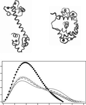
Calmodulin is the major intracellular receptor for Ca2+, and is responsible for the Ca2+-dependent regulation of a wide variety of cellular processes via interactions with a diverse array of target enzymes including a number of kinases. The Ca2+/calmodulin (CaM)-dependent activation of myosin light chain kinase (MLCK) is a model for CaM-kinase interactions that has been investigated extensively. All isoforms of MLCK include a conserved catalytic core homologous to that of other protein kinases, followed immediately by a carboxyl-terminal regulatory segment consisting of both an auto-inhibitory sequence and a CaM-binding sequence [101]. In its inhibited conformation, the regulatory segment of MLCK maintains numerous contacts with the catalytic core, thus preventing substrate binding and its subsequent phosphorylation [102–104]. CaM has an unusual dumbbell-shaped structure with two globular lobes connected by an extended helix, each having two Ca2+-binding, aka. “EF hand” motifs [105]. A ribbon representation of the peptide backbone structure of 4Ca2+-CaM from its crystal structure is shown in Fig. 8.6a. When Ca2+ binds to calmodulin, hydrophobic clefts on each globular lobe that are important in target enzyme recognition and binding are exposed (reviewed in [106, 107]).

Small-angle X-ray and neutron scattering [14] were the first experiments to demonstrate that CaM undergoes a dramatic conformational collapse upon binding a 25 amino acid peptide with a sequence homologous to the CaMbinding region from MLCK. Figure 8.6c shows the P (r) that was determined from a SANS “solvent-matching” experiment on perdeuterated CaM and a nondeuterated MLCK-I peptide in a bu er containing 37% D2O. Deuterated calmodulin has a neutron SLD that is greater than that of 100% D2O, while the nondeuterated peptide has a SLD approximately equal to that of the bu er in 37% D2O. Thus, in the 37% D2O bu er, deuterated CaM is strongly contrasted against the solvent but nondeuterated MLCK-I peptide has the same mean SLD as the solvent and hence does not contribute to the scattering. The maximum linear dimension of CaM in the complex (where the

˚	˚	for CaM without the
P (r) goes to zero) is approximately 50 Aversus 68 A

peptide present, which could only be achieved if the two globular domains of CaM come into close contact. This observed collapse of CaM was proposed to be achieved via flexibility in the interconnecting helix region that

150 J.K. Krueger et al.

(a)

(b)

(c)

P (r)

0.5

0.4

0.3

0.2

0.1

0.0

0

10

20

30

40

50

60

70

r (Å−1)

Fig. 8.6. (a) Ribbon representation of the backbone structure of CaM in the crystal structure [16] and (b) in its complex with the peptide MLCK-I derived from the NMR data [15]. (c) P (r) functions, each scaled to the square of the molecular weight, calculated from the crystal structure of 4Ca2+/CaM (solid line) and measured using solution scattering from CaM (dashed line), 4Ca2+/CaM (open circles), and the solvent-matched 4Ca2+/CaM from the neutron scattering experiment on perdeuterated CaM bound to the MLCK-I peptide (closed circles)

allows the two lobes of the dumbbell-shaped CaM to come into close contact, encompassing the peptide as the hydrophobic clefts in the globular lobes of CaM interact with hydrophobic residues in the helical target peptide. Later, this collapse was confirmed and further detailed by higher resolution studies using NMR [108] (see Fig. 8.6b) and X-ray crystallography [16] on complexes of CaM with isolated peptides based on CaM-binding sequences from smooth and skeletal muscle MLCKs.

8.4.2 Contrast Variation of Deuterated CaM Bound to MLCK enzyme

It has been proposed that the regulatory segment of MLCK, which includes both autoinhibitory and CaM-recognition sequences, folds back on the

8 SANS from Biological Molecules

151

catalytic core to inhibit kinase activity [104]. This idea is consistent with the crystal structure of the autoinhibited form of CaM-dependent protein kinase I [109]. In addition, selected-site mutagenesis studies collectively show that the autoinhibitory sequence of MLCK forms an extensive network of contacts with the surface of the catalytic core [102, 103, 110]. The e ect of CaMbinding to MLCK had been proposed to involve release of autoinhibition of the kinase via some sort of movement of the autoinhibitory sequence [111, 112]. Neutron scattering studies with contrast variation provided the first direct structural evidence in support of the autoinhibitory hypothesis for MLCK activation [113].

While there has been an abundance of structural data on calmodulin– peptide complexes, until the neutron scattering contrast variation studies mentioned herein, there was very little structural data on CaM complexed with a functional enzyme. Specifically, in the case of the CaM–MLCK interactions, this situation led to speculation about whether the MLCK C-terminal regulatory region could be released from its interactions with the surface of the catalytic core such that the CaM-binding sequence would be sterically unrestricted and able to form the tight interaction with the conformationally collapsed CaM as was observed for the CaM–peptide structures. SANS contrast variation experiment on the complex formed between deuterium-labeled CaM bound to a catalytically active MLCK revealed the surprising answer. The basic scattering functions for the individual components of each complex were extracted from the contrast series yielding the Rg and P (r) distributions for the CaM and MLCK components as well as the distances between the centers of mass of the two components in each complex. The results showed that indeed CaM undergoes an unhindered conformational collapse upon binding MLCK that is very similar to that observed with the isolated CaMbinding peptides. An MC integration modeling procedure, BIOMOD [114], was used to systematically test against the scattering data all possible twoellipsoid uniform-density models for the complex within the set constrained by the known structural parameters. Figure 8.7 (left) shows the resultant twoellipsoid model of the scattering data that led to an autoinhibitory hypothesis for MLCK activation. It was clear from the model that CaM binding to the enzyme must induce a significant movement of the kinase’s CaM-binding and autoinhibitory sequences away from the surface of the catalytic core. Major factors that were critical to the success of this contrast variation experiments include: (i) working at low concentrations ( 1 – 2 mg ml) to avoid time-dependent aggregation of the complex, (ii) collecting a complete contrast series to extract basic scattering functions as the concentration of the CaM component was so low that the 40% D2O solvent-matched contrast was very weak, and thus, (iii) the higher intensity of the neutron beam as a result of the cold source upgrade at NIST [37].

Neutron contrast series data were collected for deuterated CaM bound to MLCK in the presence of substrates (a nonhydrolyzable analog of adenosine triphosphate, AMPPNP, and a peptide substrate that includes the