Ersoy O.K. Diffraction, Fourier optics, and imaging (Wiley, 2006)(ISBN 0471238163)(427s) PEo

108	WIDE-ANGLE NEAR AND FAR FIELD APPROXIMATIONS

1200

1000

800

600

400

200

0

0.01

	0.005	0.01
	0	0.005
		0
	–0.005
		–0.005
	–0.01
		–0.01

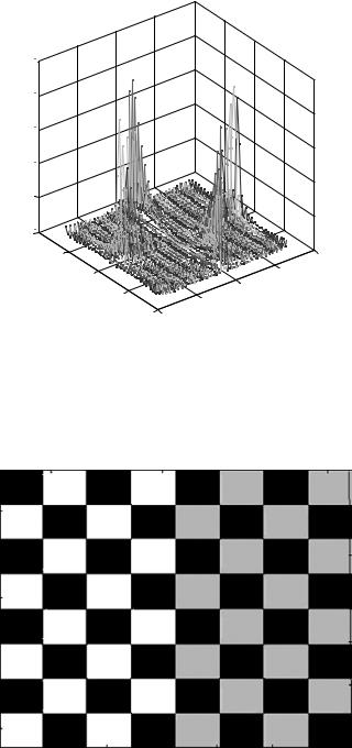
Figure 7.13. The output diffraction amplitude computed with the NFFA.

first one is by inverse Fresnel approximation given by Eqs. (7.5-1) and (7.5-2). The second one is by inverse NFFA approximation given by Eqs. (7.5-3) and (7.5-4). Figure 16 also shows the NFFA reconstruction of the output diffraction amplitude at the semi-irregularly sampled output points, meaning that it is the same as the

1200

1000

800

600

400

200

0

0.01

0.005 0.01

0

0.005

–0.005

0 –0.005

–0.01 –0.01

Figure 7.14. The output diffraction amplitude computed with the Fresnel approximation.

NUMERICAL EXAMPLES

109

5

4

3

2

1

0 0.01

0.005 0.01

0	0.005

0

–0.005

–0.005

–0.01 –0.01

Figure 7.15. The error in diffraction amplitude (absolute difference between Figs. 7.14 and 7.15).

original image. Figure 17 shows the output diffraction amplitude computed with the NFFA at the regularly sampled output points, starting with the input diffraction pattern obtained with the inverse Fresnel approximation. As the NFFA is believed to be accurate, the output diffraction amplitude in an actual physical implementation would look like Figure 17 at the regularly sampled output points.

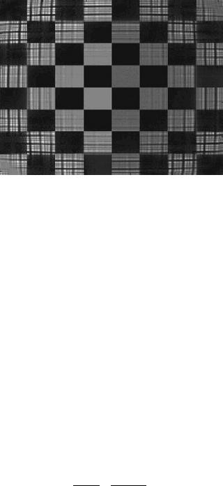
Figure 7.16. The checkerboard image and its NFFA reconstruction from the field computed with the inverse NFFA (z ¼ 80 mm, input size ¼ 0:8 0:8 mm, output size ¼ 16:2 16:2 mm).

110	WIDE-ANGLE NEAR AND FAR FIELD APPROXIMATIONS

Figure 7.17. The NFFA reconstruction of the checkerboard image from the field computed with the inverse Fresnel approximation (z ¼ 80 mm, input size ¼ 0:8 0:8 mm, output size ¼ 16:2 16:2 mm).

7.7MORE ACCURATE APPROXIMATIONS

If the output space coordinates are centered around ðxc; ycÞ, and the input space coordinates are centered around ðxI; yIÞ, better accuracy can be obtained by defining

x0 ¼ x00	þ xc	ð7:7-1Þ
y0 ¼ y00	þ yc	ð7:7-2Þ
x ¼ x0	þ xI	ð7:7-3Þ
y ¼ y0	þ yI	ð7:7-4Þ
q ¼ ðxc xIÞ2 þ ðyc yIÞ2		ð7:7-5Þ
rc ¼ ½z2 þ q&1=2		ð7:7-6Þ

The following is defined:

xcI ¼ xc xI ycI ¼ yc yI

v0 ¼ x020 þ y020 þ 2½xcIx00 þ ycIy00&

w0 ¼ x02 þ y02 2½xcIx0 þ ycIy0&

g0 ¼ v0 þ w0 x00x þ y00y 2rc2 rc2

ð7:7-7Þ

ð7:7-8Þ

ð7:7-9Þ

ð7:7-10Þ

ð7:7-11Þ

CONCLUSIONS

111

Then, the analysis remains valid with z replaced by rc and g, v, w replaced by g0, v0, w0, respectively. In this case, the error is approximately given by

v0

x2

y2

x0x

y0y

2

E

ð

þ

Þ

ð

þ

Þ

7:7-12

’

4rc3

2rc3

ð

Þ

These approximations would be especially useful in large scale simulations by dividing the input and/or output areas into smaller subareas and applying the NFFA between such subareas. With a parallel processing system, large-scale simulations can then be carried out in near real time.

7.8CONCLUSIONS

We conclude that the Fresnel and Fraunhofer approximations can be considerably improved with the NFFA, especially for wide-angle computations while still utilizing the FFT for computation by more accurately sampling the output points.

The major difference between the Fresnel/Fraunhofer approximations and the NFFA is indeed the different sampling points. The different phase factors outside the integrals in Eqs. (7.2-11) and (7.3-11) are comparable except for very wide angles of diffraction and do not affect the diffraction intensity pattern at the output plane. Hence, when the Fresnel approximation is used as it has always been, the results are still sufficiently accurate at the new sampling points determined by Eqs. (7.3-8) and (7.3-9), but now these results are really the NFFA results at the new sampling points. The new permissible z-distance in the NFFA is smaller than the permissible z-distance with the Fresnel approximation by a considerable factor such as 18.

As long as semi-irregular output point is acceptable, the NFFA can be considered to be as accurate as the angular spectrum method, but also with wide angles of diffraction, at most geometries considered in practice.

8

Geometrical Optics

8.1INTRODUCTION

Geometrical optics (ray optics) involves approximate treatment of wave propagation in which the wavelength l is considered to be infinitesimally small. In practice, this means l is much smaller than the spatial sizes of all disturbances to the amplitude or phase of a wave field. For example, if a phase shift of 2p radians occurs over a distance of many wavelengths due to a phase-shifting aperture, geometrical optics can be reliably used. For example, ray optics can be used in a large core multimode optical fiber.

In geometrical optics, a wave field is usually described by rays which travel in different optical media according to a set of rules. The Eikonal equation forms the basis of geometrical optics. It can be derived from the Helmholtz equation as the wavelength approaches zero.

This chapter consists of eight sections. Section 8.2 introduces the physical fundamentals of the propagation of rays. This is followed by the ray equation in Section 8.3. For rays traveling close to the optical axis, it is shown that the simplification of the ray equation results in the paraxial ray equation.

The eikonal equation is derived in Section 8.4. Local spatial frequencies and rays are illustrated in Section 8.5 with examples. The meridional rays, which are rays traveling in a single plane containing the optical axis and another orthogonal axis such as the y-axis, are described in Section 8.6 in terms of 2 2 matrix algebra. The theory is generalized to thick lenses in Section 8.7. The entrance and exit pupils of a complex optical system are described in Section 8.8.

8.2PROPAGATION OF RAYS

In geometrical optics, the location and direction of rays are of primary concern. For example, in image formation by an optical system, the collection of rays from each point of an object are redirected towards a corresponding point of an image.

Diffraction, Fourier Optics and Imaging, by Okan K. Ersoy

Copyright # 2007 John Wiley & Sons, Inc.

112

PROPAGATION OF RAYS

113

B

ds

A

Figure 8.1. Optical path length between A and B.

Optical components centered about an optical axis are usually small such that the rays travel at small angles. Such rays are called paraxial rays and are the basis of paraxial optics.

The basic postulates of geometrical optics are as follows:

1.A wave field travels in the form of rays.

2.A ray travels with different velocities in different optical media: the refractive index, n of an optical medium is a number greater than or equal to unity. If the velocity equals c when n equals 1, the velocity equals c/n when n 6¼ 1. n is often a function of position, say, n(r) in a general optical medium.

3.Fermat’s principle: Rays travel along the path of least-time. In order to understand this statement better, consider Figure 8.1. The infinitesimal time of travel in the differential length element ds along the path as shown in Figure 8.1 is given by

	ds		nðrÞds		8:2-1
	c=nðrÞ ¼		c	ð		Þ
We define optical path length Lp between the points A and B as
		B
	Lp ¼ ðA nðrÞds			ð8:2-2Þ

Then, the time of travel between A and B is given by Lp=c.

Fermat’s principle states that Lp is an extremum with respect to neighboring paths:

dLp ¼ 0

ð8:2-3Þ

Dividing this equation by v, the variation of travel time also satisfies

Lp	¼ 0	ð8:2-4Þ
v

This extremum is typically a minimum such that rays follow the path of least time.

114							GEOMETRICAL OPTICS

Figure 8.2. Minimum path between A and B after reflection from a mirror.

In a homogeneous medium, n is constant. Then, the path of minimum optical path length between two points is the straight line between these two points. This is often stated as ‘‘rays travel in straight lines.’’

Fermat’s principle can be used to prove what happens when a ray is reflected from a mirror, or is reflected and refracted at the boundary between two optical media, as illustrated in the following examples.

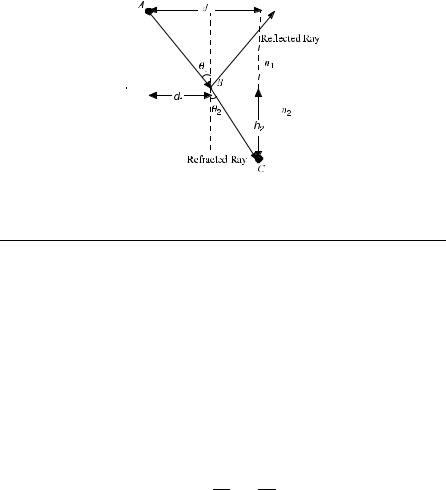
EXAMPLE 8.1 Show that when a ray reflects from a mirror, the angle of reflection should be equal to the angle of incidence in a medium of constant n.

Solution: The geometry involved is shown in Figure 8.2. y1 and y2 are the angles of incidence and of reflection, respectively. The path between A and C after reflection from the mirror should be a minimum.

The path length is given by

Lp ¼ nðAB þ BCÞ

which can be written as

Lp ¼ nð½h21 þ ðd1 d2Þ2&1=2 þ ½h22 þ d22&1=2Þ

Lp depends on d2 as the independent variable. Setting dLp=dd2 ¼ 0 yields

	d1 d2	¼	d2
	½h12 þ ðd1 d2Þ2&1=2		½h22 þ d22&1=2
which is the same as

sinðy1Þ ¼ sinðy2Þ

or

y1 ¼ y2

PROPAGATION OF RAYS	115

Figure 8.3. Reflection and refraction at the boundary between two optical media.

EXAMPLE 8.2 (a) An incident ray is split into two rays at the boundary between two optical media with indices of refraction equal to n1 and n2, respectively. This is visualized in Figure 8.3.

Show that

n1 sin y1 ¼ n2 sin y2

This is called Snell’s law.

(b) For rays traveling close to the optical axis, show that

n1y1 n2y2

ð8:2-5Þ

ð8:2-6Þ

This is called paraxial approximation in geometrical optics. Solution: (a) The optical path length between A and C is given by

Lp ¼ n1AB þ n2BC

By Fermat’s principle, Lp is to be minimized. Lp can be written as

Lp ¼ n1½h21 þ d12&1=2 þ n2½h22 þ ðd d1Þ2&1=2

The independent variable is d1. Setting dLp=dd1 ¼ 0 yields

	n1d1	¼		n2ðd d1Þ
½h12 þ d12&1=2			½h22 þ ðd d1Þ2&1=2
which is the same as

n1 sin y1 ¼ n 2 sin y2

116 GEOMETRICAL OPTICS

(b) When the rays travel close to the optical axis, sin y1 y1 and sin y2 y2 so that

n1y1 n1y2

EXAMPLE 8.3 A thin lens has the property shown in Figure 8.3.

A ray incident at an angle y1 leaves the lens at an angle y2 given by
y2 ¼ y1	y		ð8:2-7Þ
	f

where y is the distance from the optical axis, and f is the focal length of the lens given by

1	1		1
	¼ ðn 1Þ					ð8:2-8Þ
f		R1		R2

n is the index of refraction of the lens material, R1 and R2 are the radii of curvature of the two surfaces of the lens.

Using the information given above, show the lens law of image formation. Solution: Consider Figure 8.4(b). As a consequence of Eq. (8.2-7), and paraxial approximation such that sin y y, the ray starting at P1 and parallel to the optical axis passes through the focal point F since y1 equals zero; the ray starting at P1 and passing through the center point of the lens on the optical axis goes through the lens without change in direction since y equals 0. The two rays intersect at P2, which determines the image.

q1	q 2
	y
P1	P2

(a)

P1

F

P2

f

z1 z2

(b)

Figure 8.4. (a) Ray bending by a thin lens, (b) Image formation by a thin lens.

THE RAY EQUATIONS

117

	y
	x
	B
	ds
	s
x	z

Figure 8.5. The trajectory of a ray in a GRIN medium.

8.3THE RAY EQUATIONS

In a graded-index (GRIN) material, the refractive index is a function n(r) of position r. In such a medium, the rays follow curvilinear paths in accordance with Fermat’s principle.

The trajectory of a ray can be represented in terms of the coordinate functions x(s), y(s) and z(s), s being the length of the trajectory. This is shown in Figure 8.5.

The trajectory is such that Fermat’s principle is satisfied along the trajectory between the points A and B:

B
d ðA nðrÞds ¼ 0	ð8:3-1Þ

r being the position vector. Using calculus of variations, Eq. (8.3-1) can be converted to the ray equation given by

d	dr
	nðrÞ		¼ rnðrÞ	ð8:3-2Þ
ds		ds

where r is the gradient operator. The ray equation is derived rigorously in Section 8.4 by using the Eikonal equation.

The ray equation given above is expressed in vector form. In Cartesian coordinates, the component equations can be written as

d	dx		¼	@n
	n
ds		ds		@x

d	dx		¼	@n
	n
ds		ds		@y

d	dx		¼	@n
	n
ds		ds		@z

Solution of Eq. (8.3-2) is not trivial. It can be considerably simplified by using the paraxial approximation in which the rays are assumed to be traveling close to the optical axis so that ds dz. Equation (8.3-2) can then be written in terms of two