Ersoy O.K. Diffraction, Fourier optics, and imaging (Wiley, 2006)(ISBN 0471238163)(427s) PEo

118								GEOMETRICAL OPTICS
equations given by
	d						@n
			n	dx		¼		ð8:3-3Þ
dz				dz			@x
	d			dy			@n
		n				¼		ð8:3-4Þ
dz				dz			@y

Equations (8.3-3) and (8.3-4) are called the paraxial ray equations.

EXAMPLE 8.4 Show that in a homogeneous medium, rays follow straight lines. Solution: When n is constant, Eqs. (8.3-3) and (8.3-4) become

d2x d2y

dz2 ¼ dz2 ¼ 0

Hence,

x ¼ Az þ B

ð8:3-5Þ

y ¼ Cz þ D

which represent straight lines.

EXAMPLE 8.5 If n ¼ nðyÞ, show how to utilize the paraxial ray equations. Solution: Since n is not a function of x, the variation along the x direction is still given by Eq. (8.3-5). For the y-direction, Eq. (8.3-4) can be written as

d2y	¼	1 dn
dz2		n		dy

Given n(y) and the initial conditions y(0) and for y(z).

ð8:3-6Þ

dy , Eq. (8.3-6) can be solved

dz z¼0

8.4THE EIKONAL EQUATION

A monochromatic wave field traveling in a medium in which the refractive index changes slowly with respect to the wavelength has a complex amplitude, which can be approximated as

UðrÞ ¼ AðrÞe jk0SðrÞ

ð8:4-1Þ

where k0 equals the free space wave number 2p=l0, l0 is the free space wavelength, and k0SðrÞ is the phase of the wave. SðrÞ is a function of the refractive index n(r) and is called the Eikonal ( function).

Constant phase surfaces are defined by

SðrÞ ¼ constant

ð8:4-2Þ

THE EIKONAL EQUATION

119

Such surfaces are called wavefronts. Power flows in the direction of k which is perpendicular to the wavefront at a point r. The trajectory of a ray can be shown to be always perpendicular to the wavefront at every point. In other words, a ray follows the direction of power flow.

Equation (8.4-1) can be substituted in the Helmholtz equation

	ðr2 þ k2ÞUðrÞ ¼ 0							ð8:4-3Þ
	to yield
	k02½n2 jrSj2&A þ r2A ¼ 0							ð8:4-4Þ
	and
	k0½2rS rA þ Ar2S& ¼ 0							ð8:4-5Þ
	Equation (8.4-4) is rewritten as
	S	2		n2		l02	r2A	ð	8:4-6	Þ
		j	¼		þ 2p2 A
	jr

As l0 ! 0, the second term on the right-hand side above can be neglected so that

jrSðrÞj2 n2ðrÞ

ð8:4-7Þ

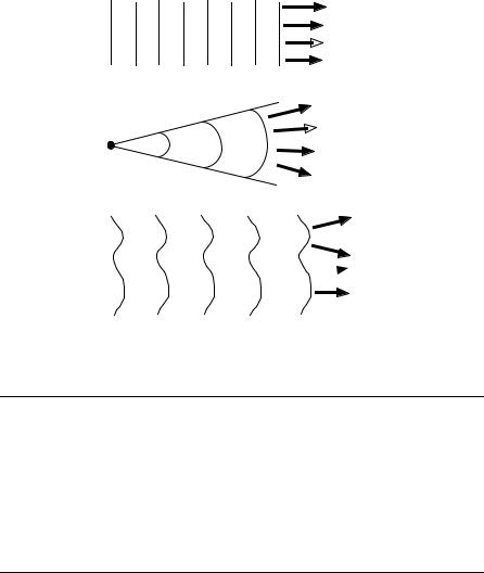
Equation (8.4-7) is known as the Eikonal equation. It can be used to determine wavefronts. Once the wavefronts are known, the ray trajectories are determined as being perpendicular to the wavefronts. Three types of wavefronts are shown in Figure 8.6.

The Eikonal equation can be interpreted as the limit of the Helmholtz equation as the wavelength approaches zero.

Once S(r) is obtained by using Eq. (8.4-7), A(r) can be determined by using Eq. (8.4-5). Thereby, the wave field U(r) is known.

Equation (8.4-7) can also be written as

	@S		2		@S 2			@S		2
				þ			þ			¼ n2ðrÞ	ð8:4-8Þ
	@x				@y			@z

Then, the index of refraction is given by

nðrÞ ¼ jrSðrÞj

ð8:4-9Þ

120	GEOMETRICAL OPTICS

Rays

(a)

Rays

(b)

Rays

(c)

Figure 8.6. Three types of wavefronts: (a) a plane wave, (b) a spherical wave, (c) a general wave.

EXAMPLE 8.6 Show that the optical path length between two points A and B equals SðrBÞ SðrAÞ.

Solution: Since nðrÞ ¼ jrSðrÞj, the optical path length is given by

B	B
Lp ¼ ðA nðrÞdr ¼	ðAjrSðrÞjdr ¼ SðrBÞ SðrAÞ

Note that the optical path length is similar to potential difference in electrostatics. Then, the phase S(r) is analogous to potential at a point.

8.5LOCAL SPATIAL FREQUENCIES AND RAYS

In previous chapters, an arbitrary wave was analyzed in terms of plane wave components with direction cosines. Optical rays can also be associated with direction cosines. In order to do so, it is necessary to consider the nonstationary characteristics of a wave field.

In general, a nonstationary signal h(t) is a signal whose frequency content changes as a function of t. Such signals are not well characterized by a single Fourier transform representation. Instead a short-time Fourier transform can be used by computing the Fourier transform of hðtÞoðtÞ, oðtÞ being a window function of limited extent.

LOCAL SPATIAL FREQUENCIES AND RAYS

121

The 1-D case outlined above can be generalized to the 2-D case in terms of nonstationary 2-D signals, which is relevant to wave fields. Thus, let us write a wave field at constant z as

hðx; yÞ ¼ Aðx; yÞejfðx;yÞ						ð8:5-1Þ
where z is suppressed. A(x,y) will be assumed to be slowly varying.
The local spatial frequencies are defined by
fx0	¼	1 @			fðx; yÞ	ð8:5-2Þ
		2p		@x
fy0	¼	1 @			fðx; yÞ	ð8:5-3Þ
		2p		@y

fx0 and fy0 are also defined to be zero in regions where h(x,y) is zero.

In general, fx0 and fy0 are not the same as the Fourier transform spatial frequencies fx and fy discussed in previous chapters. Good agreement between the two sets occurs only when the phase fðx; yÞ varies slowly in the x–y plane so that fðx; yÞ can be approximated by three terms of its Taylor series expansion near any point (x0,y0).

The terms involved are fðx0; y0Þ,

@

@

@x

fðx; yÞ xy¼¼yx00

and

@y

fðx; yÞ xy¼¼yx00

:

The local direction cosines

are defined by

a0 ¼ lfx0

ð8:5-4Þ

b0 ¼ lfy0

ð8:5-5Þ

g0

q

8:5-6

¼

ð

Þ

It can be shown that these direction cosines are exactly the same as the direction cosines of a ray at (x,y) on a plane defined by constant z.

EXAMPLE 8.7 Determine the local spatial frequencies of a plane wave field. Solution: The spatial part of a plane wave field can be written as

hðx; yÞ ¼ ej2pðfx xþfyyÞ

Then, with fðx; yÞ ¼ 2p fxx þ fyy

fx0 ¼ 21p @@x fðx; yÞ ¼ fx fy0 ¼ 21p @@y fðx; yÞ ¼ fy

122	GEOMETRICAL OPTICS

In this case, the local spatial frequencies and the Fourier transform spatial frequencies are the same.

EXAMPLE 8.8 A finite chirp function is defined by

2	2	Þrect	x	rect	y
hðx; yÞ ¼ ejpaðx	þy
			2Dx		2Dy

(a)Determine the local spatial frequencies.

(b)Compare the local frequencies to the properties of the Fourier transform of

g(x,y).

Solution: (a) The phase is given by

fðx; yÞ ¼ paðx2 þ y2Þ

in a rectangular region around the origin of dimensions 2Dx by 2Dy. In this region, the local spatial frequencies are given by

fx0	¼	1		@		fðx; yÞ ¼ ax
			2p		@x
fy0	¼	1		@		fðx; yÞ ¼ ay
			2p		@y

Outside the rectangular region, fx0 and fy0 are zero by definition. Hence, they can be

written as
fx0	¼ ax rect	x
		2Dx
fy0	¼ ax rect	y
		2Dy

Note that fx0 and fy0 vary linearly with x and y, respectively, inside the given rectangular region.

(b) h(x,y) is a separable function:		rect 2DX		ejpay	rect 2Dy
hðx; yÞ ¼ h1ðxÞh2ðyÞ ¼ ejpax
	2		x	2		y
Hence, the Fourier transform of h(x,y) equals H1ðfxÞH2ðfyÞ.
The Fourier transform of h1(x) is given by
	Dx
H1ðfxÞ ¼	ð	ejpax2 e j2pfxxdx			ð8:5-7Þ

Dx

MATRIX REPRESENTATION OF MERIDIONAL RAYS

123

¼

p

ð

ð

ÞÞ

Let v

2a x

fx=a . Then, Eq. (8.5-7) can be written by change of variables as

L2

1

2

ð

pv2

1

2

pfx

pfx

H1

ðfxÞ ¼ p2a e j

a

ej

2 dv ¼ p2a e j

a

½CðL2Þ CðL1Þ þ jSðL2Þ jSðL1Þ&

L1

ð8:5-8Þ

where C(.) and S(.) are the Fresnel cosine and sine integrals given by Eqs. (5.2-18) and (5.2-19), and L1, L2 are defined by

L1 ¼ p2a Dx þ	fx		ð8:5-9Þ
	a
L2 ¼ p2a Dx	fx		ð8:5-10Þ
	a

H2ðfyÞ is similarly computed. It can be shown that the amplitude of H1ðfxÞ fast approaches zero outside the rectangular region [Goodman, 2004]. In other words, the frequency components are negligible away from the rectangular region. The fact that local frequencies are zero outside the rectangular region also suggests the same result. However, similarity between local frequencies and Fourier frequencies is not easy to show in more complicated problems.

8.6MATRIX REPRESENTATION OF MERIDIONAL RAYS

Meridional rays are rays traveling in a single plane containing the z-axis called the optical axis. The transverse axis can be called the y-axis. Under the paraxial approximation ðsin y yÞ, rays traveling in such a plane can be characterized in terms of a 2 2 matrix called the ray-transfer matrix.

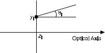
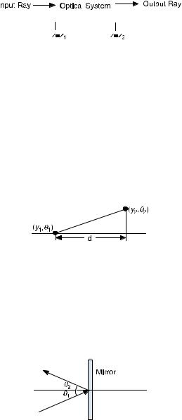
A meridional ray at z ¼ zi in the paraxial approximation is characterized by its position yi and angle yi, as shown in Figure 8.7. This will be denoted as a pair ðyi; yiÞ. Consider the traveling of the ray within an optical system from z ¼ z1 to z ¼ z2 as shown in Figure 8.8.

Figure 8.7. A ray at z ¼ zi characterized by (yi ; yi).

124				GEOMETRICAL OPTICS

Figure 8.8. The travel of a ray through an optical system between z ¼ z1 and z ¼ z2.

In the paraxial approximation, ðy1; y1Þ and ðy2; y2Þ are related by

y2	¼	C D	y1	ð8:6-1Þ
y2		A B	y1

where the matrix M with elements A, B, C, D is called the ray-transfer matrix. The ray transfer matrices of elementary optical systems are discussed below.

1.Propagation in a medium of constant index of refraction n: This is as shown in Figure 8.9.

Figure 8.9. Propagation in a medium of constant index of refraction n.

M is given by

M ¼	1	d	ð8:6-2Þ
	0	1

2. Reflection from a planar mirror: This is as shown in Figure 8.10.

Figure 8.10. Reflection from a planar mirror.

M is given by

M ¼	1	0	ð8:6-3Þ
	0	1

MATRIX REPRESENTATION OF MERIDIONAL RAYS

125

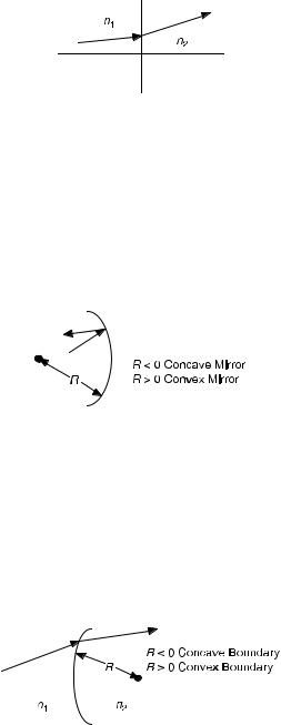
3. Refraction at a planar boundary: This is as shown in Figure 8.11.

Figure 8.11. Refraction at a plane boundary.

M is given by

1	0	5
4	n2
M ¼ 2 0	n1	3	ð8:6-4Þ

4. Reflection from a spherical mirror: This is as shown in Figure 8.12.

Figure 8.12. Reflection from a spherical mirror.

M is given by

	1	0
4 R		5
M ¼ 2	2	1 3	ð8:6-5Þ

5. Refraction at a spherical boundary: This is as shown in Figure 8.13.

Figure 8.13. Refraction at a spherical boundary.

126						GEOMETRICAL OPTICS
M is given by
M ¼		1	0n1		3	ð8:6-6Þ
	2 n1 n2
	4				5
		n2R	n2

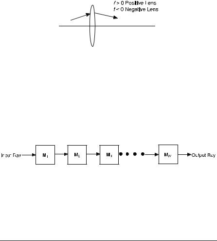
6. Transmission through a thin lens: This is as shown in Figure 8.14.

Figure 8.14. Transmission through a thin lens.

M is given by

M ¼	2 1		1	01	3	ð8:6-7Þ
	4	f			5

7.Cascaded optical components: Suppose N optical components are cascaded, as shown in Figure 8.15.

Figure 8.15. Transmission through N optical components.

The ray-transfer matrix for the total system is given by

M ¼ MN MN 1 M1

ð8:6-8Þ

EXAMPLE 8.9 Show that the ray-transfer matrix for a thin lens is given by Eq. (8.6-7).

Solution: A thin lens with an index of refraction n2 has two spherical surfaces with radii R1 and R2, respectively. Suppose that the index of refraction outside the lens

MATRIX REPRESENTATION OF MERIDIONAL RAYS

127

equals n1. Transmission through the lens involves refraction at the two spherical surfaces. Hence, the total ray-transfer matrix is given by

M ¼ M2M1	¼	2 n2 n1			n2	32 n1 n2			n1 3		¼	2	1		1	3
		1		0		1		0					1		0
		4				54				5		4				5
			n1R2		n1		n2R1		n2
														f

where the focal length f is determined by

1		n2 n1		1		1
	¼
f			n1		R1		R2

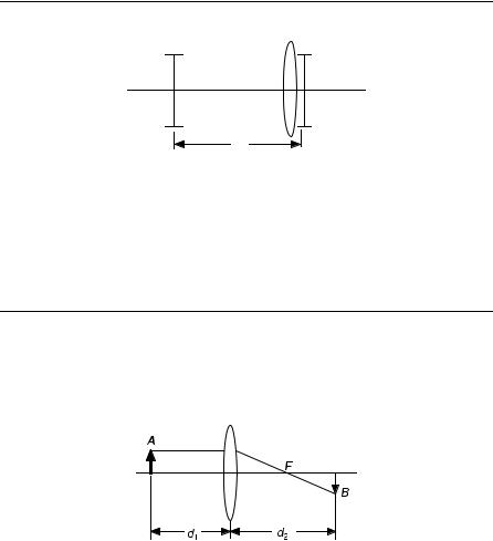
EXAMPLE 8.10 Determine the ray-transfer matrix for the following system:

Input

Output

d

Solution: The system is a cascade of free-space propagation at a distance d and transmission through a thin lens of focal length f. Hence, the ray-transfer matrix is given by

	1		0	1	d		1			d
4	f		5			4	f			f		5
M ¼ M2M1 ¼ 2	1		1 3 0		1 2		1		1	d		3

EXAMPLE 8.11 (a) Derive the imaging equation for a single thin lens of focal length f, (b) determine the magnification.

Solution: The object is assumed to be at a distance d1 from the lens; the image forms at a distance d2 from the lens as shown in Figure 8.16.

Figure 8.16. Imaging by a single lens.