Ersoy O.K. Diffraction, Fourier optics, and imaging (Wiley, 2006)(ISBN 0471238163)(427s) PEo

158	IMAGING WITH QUASI-MONOCHROMATIC WAVES
The analytic signal can be further written as
sðtÞ ¼ jsðtÞje jfðtÞ						ð10:3-5Þ
where
jsðtÞj2 ¼ u2ðtÞ þ v2ðtÞ						ð10:3-6Þ
t	Þ ¼	tan 1	vðtÞ			ð	10:3-7	Þ
fð			u t	Þ
		ð

The analytic signal is often used with narrowband waveforms such as quasimonochromatic wave fields with central frequency fc. Then, fðtÞ can be written as

fðtÞ ¼ 2pfct þ f0ðtÞ	ð10:3-8Þ
Equation (10.2-13) can be written as
sðtÞ ¼ mðtÞe j2pfct	ð10:3-9Þ
where
mðtÞ ¼ jsðtÞje jf0ðtÞ	ð10:3-10Þ

mðtÞ is called the complex envelope. In optics, it is also referred to as the phasor amplitude.

EXAMPLE 10.4 Find the analytic signal corresponding to uðtÞ ¼ cosð2pftþ fðf ÞÞ. Solution: In Example 1.25, we found that

vðtÞ ¼ sinð2pft þ fð f ÞÞ	ð10:3-11Þ
Hence,
sðtÞ ¼ cosð2pftÞ þ j sinð2pftÞ ¼ e j2pft	ð10:3-12Þ

EXAMPLE 10.5 Find the energy in the analytic signal.

Solution: The energy of the analytic signal is

1		1		1		1	1
ð	jsðtÞj2dt ¼	ð	u2ðtÞdt þ	ð	v2ðtÞdt ¼ 2	ð	u2ðtÞdt ¼ 2 ð	jUð f Þj2df
1		1		1		1	1

ð10:3-13Þ

ANALYTIC SIGNAL

159

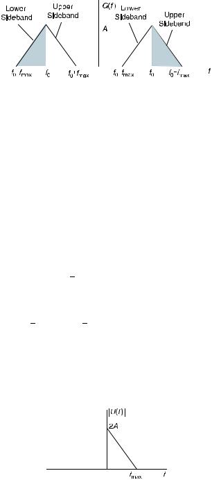
Figure 10.1. The spectrum of a lowpass signal.

It is observed that the analytic signal has twice the energy of the corresponding real signal.

EXAMPLE 10.6 The amplitude spectrum of a lowpass signal uðtÞ is shown in Figure 10.1.

It is modulated by cosð2pf0tÞ to generate gðtÞ ¼ uðtÞ cosð2pf0tÞ. (a) Find and draw the amplitude spectrum of gðtÞ, and (b) Draw the amplitude spectrum of the analytic signal generated from uðtÞ, and (c) Find and draw the amplitude spectrum of pðtÞ ¼ uðtÞ cosð2pf0tÞ vðtÞ sinð2pf0tÞ.

Solution:

(a) gðtÞ can be written as

g t

Þ ¼

uðtÞ

e j2pf0t

þ

uðtÞ

e j2pf0t

ð

10:3-14

Þ

ð

2

2

The FT of gðtÞ is given by

Gð f Þ ¼

1

Uð f f0

Þ þ

1

Uð f þ f0

Þ

ð10:3-15Þ

2

2

The amplitude spectrum is given by

1

jUð f f0Þ þ Uð f þ f0Þj

jGð f Þj ¼

ð10:3-16Þ

2

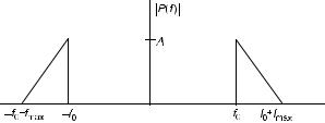
jGð f Þj is shown in Figure 10.2.

and f0 fmax

The frequency components in the range f0 f f0 þ fmax

f f0 are known as the upper sideband. The frequency components in the range

f0 f f0 þ fmax and f0 fmax f f0 are known as the lower sideband.

(b) The analytic signal generated from u(t) is given by

sðtÞ ¼ uðtÞ þ jvðtÞ

ð10:3-17Þ

160

IMAGING WITH QUASI-MONOCHROMATIC WAVES

Figure 10.2. The amplitude spectrum of Gðf Þ.

Its FT is

Sð f Þ ¼ Uð f Þ þ jVð f Þ

¼ Uð f Þ½1 þ jHð f Þ&

(

¼	2Uð f Þ	f 0
	0	f < 0

The amplitude spectrum of s(t) is shown in Figure 10.3.

(c) pðtÞ ¼ uðtÞ cosð2pf0tÞ vðtÞ sinð2pf0tÞ can be written as

pðtÞ ¼ Re½ðuðtÞ þ jvðtÞÞe j2p f0t&

¼Re½sðtÞe j2p f0t&

¼1 ½sðtÞe j2p f0t þ s ðtÞe j2p f0t&

2

The FT of pðtÞ can be written as

Pð f Þ ¼ 12 Sð f f0Þ þ 12 S ð f f0Þ

8

> Uð f f0Þ f0 f f0 þ fmax

>

<

¼> U ð f f0Þ f0 fmax f f0

>

: 0 otherwise

ð10:3-18Þ

ð10:3-19Þ

ð10:3-20Þ

Figure 10.3. The amplitude spectrum of the analytic signal sðtÞ.

ANALYTIC SIGNAL REPRESENTATION OF A NONMONOCHROMATIC WAVE FIELD 161

Figure 10.4. The amplitude spectrum of the single sideband signal pðtÞ.

The amplitude spectrum of pðtÞ is shown in Figure 10.4.

pðtÞ is known as the single sideband signal because it contains only the upper sideband of uðtÞ. If it was chosen instead as uðtÞ cosð2pf0tÞ þ vðtÞ sinð2pf0tÞ, it would contain the lower sideband only. In this way, the frequency bandwidth required to transmit the signal over a channel is reduced by a factor of 2.

10.4 ANALYTIC SIGNAL REPRESENTATION OF A NONMONOCHROMATIC WAVE FIELD

Let uðr; tÞ represent the real representation of a nonmonochromatic wave field. As discussed in Section 2.7, uðr; tÞ can be written in Fourier representation as

	1
uðr; tÞ ¼ 2	ð Uðr; f Þ cosð2p ft þ fð f Þd f	ð10:4-1Þ

0

where Uðr; f Þ and fð f Þ are the amplitude and phase spectra of uðr; tÞ with respect to t, respectively.

The analytic signal corresponding to uðr; tÞ is given by

uAðr; tÞ ¼ uðr; tÞ þ jvðr; tÞ

ð10:4-2Þ

where vðr; tÞ is the Hilbert transform of uðr; tÞ. As the Hilbert transform of cosð2pft þ fð f ÞÞ equals sinð2pft þ fð f ÞÞ by Example 10.1, vðr; tÞ can be written as

	1
vðr; tÞ ¼ 2	ð0	Uðr; f Þ sinð2p ft þ fð f ÞÞdf	ð10:4-3Þ
Hence, the analytic signal uAðr; tÞ is given by
		1
		ð
uAðr; tÞ ¼ 2 Uðr; f Þejð2pftþfð f ÞÞdf			ð10:4-4Þ

0

162	IMAGING WITH QUASI-MONOCHROMATIC WAVES

Note that Ucðr; f Þ ¼ 12 Uðr; f Þe jfðf Þ is the Fourier transform of uðr; tÞ with respect to t. Equation (10.4-4) shows that the analytic signal is obtained by integrating the spectrum of the original signal over positive frequencies only. uðr; tÞ can also be written as

uðr; tÞ ¼	1	½sðr; tÞ þ s ðr; tÞ&	ð10:4-5Þ
	2

In the context of waves, the analytic signal is often referred to as the complex wave function [Saleh and Teich, 1991].

10.5 QUASI-MONOCHROMATIC, COHERENT, AND INCOHERENT WAVES

A wave field is called quasi-monochromatic if its temporal frequency spread f satisfies

f	1	ð10:5-1Þ
fc

where fc is the mean temporal frequency of the wave field. In this case, uAðr; tÞ can be written as

uAðr; tÞ ¼ UAðr; tÞe j2p fct

ð10:5-2Þ

where UAðr; tÞ is the complex envelope of the analytic signal.

A wave field that is monochromatic is perfectly coherent. The subject of coherence of wave fields is very broad. For example, see references [Born and Wolf, 1969] and [Marathay]. A coherent wave field is characterized by its ability to generate constructive and destructive interference on a time-average basis when its different portions are combined at the same point.

Coherence is usually discussed in terms of spatial coherence and temporal coherence. Let uAðr; tÞ be the analytic signal representation of a wave field. If uAðr1; tÞ and uAðr2; tÞ are related by a complex constant factor independent of time for all points r1 and r2, the wave field is called spatially coherent. In the following sections, spatially coherent waves are simply referred to as coherent waves.

If the relationship between uAðr; t1Þ and uAðr; t2Þ depends only on the time difference t2 t1, the wave field is temporally coherent.

10.6DIFFRACTION EFFECTS IN A GENERAL IMAGING SYSTEM

In Section 9.4, image formation with a single lens was discussed as 2-D linear filtering. It is possible to generalize the results obtained to more general imaging

DIFFRACTION EFFECTS IN A GENERAL IMAGING SYSTEM							163

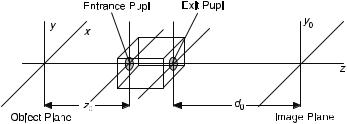
Figure 10.5. Model of an optical imaging system.

systems as well as to quasi-monochromatic sources with spatially coherent and spatially incoherent illumination.

A general imaging system typically consists of a number of lenses. Such an imaging system can be characterized in terms of an entrance pupil and an exit pupil, which are actually both images of an effective system aperture [Goodman]. This is shown in Figure 10.5. Diffraction effects can be expressed in terms of the exit pupil and the distance d0 between the exit pupil and the image plane.

An optical system is called diffraction limited if a diverging spherical wave incident on the entrance pupil is mapped into a converging spherical wave at the exit pupil. For a real imaging system, this property is at best limited to finite areas of object and image planes. Aberrations are distortions modifying the spherical property. They are discussed in Section 10.9.

In a general imaging system with many lenses, Eqs. (9.4-17) and (9.4-18) remain valid provided that P(.,.) denotes the finite equivalent exit pupil of the system, the equivalent focal length of the system and the distance from the exit pupil to the image plane is used, and the system is diffraction limited [Goodman].

We define the ideal image appearing in Eq. (8.4-17) as
	x		y
Ugðx; yÞ ¼ U		;			ð10:6-1Þ
	M		M

where Uðx; yÞ is the original image (wave field). Equation (9.4-16) is rewritten as

	1	1
Uðx0; y0Þ ¼	ð	ð	hðx0 x; y0 yÞUgðx; yÞdxdy			ð10:6-2Þ
	1 1
where
	1	1
hðx; yÞ ¼	ð	ð	Pðx1; y1Þe j	2p	ðxx0þyy0Þdxdy	ð10:6-3Þ
				ld0
	1 1

164	IMAGING WITH QUASI-MONOCHROMATIC WAVES

10.7IMAGING WITH QUASI-MONOCHROMATIC WAVES

In practical imaging systems, the conditions for quasi-monochromatic wave fields are usually satisfied. For example, in ordinary photography, films are sensitive to the visible range of the electromagnetic temporal spectrum. Then, it can be shown that the complex envelope of the analytic signal satisfies the imaging equations derived previously. Thus, Eq. (10.6-2) can be written as

UAðx0; y0; d0; tÞ ¼ hðx0; y0Þ UGðx0; y0; t tÞ

¼	ðð	hðx0 x; y0 yÞUGðx; y; t tÞdxdy ð10:7-1Þ
	1
	1

where hðx0; y0Þ is given by Eq. (10.6-3) except that l is replaced by lc, and UGðx0; y0; tÞ is the complex envelope of the analytic signal corresponding to the ideal image Uð xM0 ; yM0 ; tÞ predicted by geometrical optics; t is a time delay associated with propagation to the image plane.

The amplitude transfer function Hðfx; yyÞ is the FT of hðx; yÞ:

Hð fx; fyÞ ¼ Pðld0 fx; ld0 fyÞ

ð10:7-2Þ

Detector systems are sensitive to intensity of the wave field, which can be written as

Iðx0; y0; d0Þ ¼ hjUAðx0; y0; d0; tÞj2i

ð10:7-3Þ

where h i indicates an infinite time average. Using Eq. (10.7.1), Iðx0; y0; d0Þ can be written as

Iðx0; y0; d0Þ	ðð
ðð
1	1

¼hðx0 x; y0 yÞ h ðx0 x0; y0 y0ÞIGðx; y; x0; y0Þdx0dy0 dxdy

1	1	ð10:7-4Þ
where
	IGðx; y; x0; y0Þ ¼ hUGðx; y; t t1ÞUGðx0; y0; t t2Þi	ð10:7-5Þ

IG is known as the mutual intensity. In Eq. (10.7-5), t1 and t2 are approximately equal because the impulse response h is limited to a small region around the image point and hence can be neglected.

IMAGING WITH QUASI-MONOCHROMATIC WAVES

165

10.7.1Coherent Imaging

For perfectly coherent wave fields, we can write

UGðx; y; tÞ ¼ UGðx; yÞUGð0; 0; tÞ

ð10:7:1-1Þ

where UGðx; yÞ is the phasor amplitude of UGðx; y; tÞ relative to the wave field at the origin.

We write

		hUGðx; y; tÞUGðx; y; tÞi ¼ KUGðx; yÞUGðx0; y0Þ	ð10:7:1-2Þ
where the constant K is given by
		K ¼ hjUGð0; 0; tÞj2i	ð10:7:1-3Þ
Neglecting K, the intensity is written as
		Iðx0; y0; d0Þ ¼ jU1ðx0; y0Þj2	ð10:7:1-4Þ
where		; y0Þ ¼ hðx0; y0Þ UGðx0; y0Þ ¼ ðð hðx0 x; y0 yÞUGðx; yÞdxdy
U1	ðx0
		1

1

ð10:7:1-5Þ

Thus, the coherent imaging system is linear in complex amplitude of the analytic signal relative to the origin.

EXAMPLE 10.7 Determine the cutoff frequency of a diffraction-limited coherent imaging system with a circular effective pupil of radius R, assuming that the image forms at a distance d0 from the system.

Solution: The pupil function in this case is given by

p!

x2 þ y2

Pðx; yÞ ¼ circ

R

The amplitude transfer function is given by

H fx; fy	P ld0fx; ld0fy		circ		q
				@	fx2 þ fy2		A
					l	0
ð	Þ ¼ ð	Þ ¼		0	R= d		1

166	IMAGING WITH QUASI-MONOCHROMATIC WAVES

Hence, the cutoff frequency fc is given by

R fc ¼ ld0

10.7.2Incoherent Imaging

When the wave field is perfectly incoherent UGðx; y; tÞ is spatially uncorrelated (equivalent to white noise). Hence, the time average can be written as

hUGðx; y; tÞUGðx0; y0; tÞi ¼ KIGðx; yÞdðx x0; y y0Þ

ð10:7:2-1Þ

where IGðx; yÞ ¼ hjUGðx; y; tÞj2i. Neglecting K, Eq. (10.7-4) becomes

Iðx0; y0; d0Þ ¼	ðð	jhðx0 x; y0 yÞj2IGðx; yÞdxdy	ð10:7:2-2Þ
	1
	1

We conclude that when the wave field is incoherent, the imaging system is linear in

intensity. The ideal image intensity is filtered with the impulse response function jhðx; yÞj2.

10.8 FREQUENCY RESPONSE OF A DIFFRACTION-LIMITED IMAGING SYSTEM

In the previous section, coherent and incoherent imaging was considered as linear systems whose input is the ideal image in amplitude or intensity and whose output is the actual image, which is the convolution of the input with a system impulse response. This is shown in Figure 10.6. In this section, the system properties of coherent and incoherent imaging are studied in more detail.

10.8.1Coherent Imaging System

A coherent imaging system is linear in amplitude mapping. Let us denote the 2-D FT of the output image U1 and the ideal image UG as V1 and VG, respectively. Then, by convolution theorem,

V1ð fx; fyÞ ¼ Hð fx; fyÞVGð fx; fyÞ

ð10:8:1-1Þ

Ideal ImageLinear System Actual Image

Figure 10.6. Linear system interpretation of coherent and incoherent imaging.

FREQUENCY RESPONSE OF A DIFFRACTION-LIMITED IMAGING SYSTEM

167

where Hð fx; fyÞ is the 2-D FT of the impulse response:

Hð fx; fyÞ ¼	ðð	hðx; yÞe j2pð fxxþfyyÞdxdy ¼ Pðld0 fx; ld0 fyÞ	ð10:8:1-2Þ
	1

1

Hð fx; fyÞ is known as the coherent transfer function.

It is observed that a coherent imaging system is equivalent to an ideal low-pass filter, which passes all frequencies within the pupil function’s ‘‘1’’ zone and cuts off all frequencies outside this zone.

10.8.2Incoherent Imaging System

Incoherent imaging systems are linear in intensity. The visual quality of an image is largely determined by the contrast of the relative intensity of the informationbearing details of the image to the ever-present background. The output image and the input ideal image can be normalized by the total image energy to reflect this property:

I0ðx0	; y0; d0	Þ ¼	1	Iðx0; y0; d0Þ
			ðð Iðx0; y0; d0Þdx0dy0
		1		ð10:8:2-1Þ
	IG0 ðx; yÞ ¼		1	IGðx; yÞ
			ðð IGðx; yÞdxdy
		1

Let us denote the 2-D FT of I0ðx0; y0; d0Þ and IG0 ðx; yÞ by Jð fx; fyÞ and JGð fx; fyÞ, respectively. By convolution theorem, Eq. (10.7.2-2) can be written as

Jð fx; fyÞ ¼ HI ð fx; fyÞJGð fx; fyÞ				ð10:8:2-2Þ
where	ðð	jhðx; yÞj2e j2pð fxxþfyyÞ
	1
HI ð fx; fyÞ ¼	1 1		dxdy	ð10:8:2-3Þ
		ðð	jhðx; yÞj2dxdy
		1

HI ð fx; fyÞ is called the optical transfer function (OTF). The modulation transfer function (MTF) is defined as jHI ð fx; fyÞj.