Ersoy O.K. Diffraction, Fourier optics, and imaging (Wiley, 2006)(ISBN 0471238163)(427s) PEo

98	WIDE-ANGLE NEAR AND FAR FIELD APPROXIMATIONS

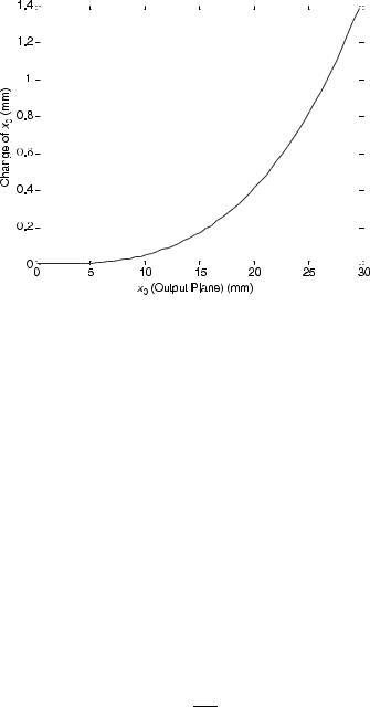
Figure 7.1. Minimum z distance for the approximations to be valid as a function of x0 at the output plane with x equal to 1 mm.

interval. Hence, the new approximation is sufficiently accurate at all the output sampling points for x=l greater than 2. Figure 7.3 shows the growth of the difference between x0 and xs calculated with Eq. (28) as x0 increases when z ¼ 10 cm.

Figure 7.2.

The ratio z=x0

as a function of x0.

NUMERICAL EXAMPLES		99

Figure 7.3. Change of x0 in mm as a function of x0 at the output plane when z ¼ 20 cm and x ¼ 1 mm.

Equations (7.3-8) and (7.3-9) show the relationship with the regularly sampled output points as in the Fresnel or Fraunhofer approximations, and the semiirregularly sampled output points as in the NFFA. Examples of these relationships are given in Tables 7.1 thru 7.3. The (x,y) sampling coordinate values in these tables are shown as complex numbers x þ iy. Table 7.1 shows the example of regularly sampled values. Table 7.2 shows the corresponding example of semi-irregularly sampled values. Table 7.3 is the difference between Tables 7.1 and 7.2.

In the next set of experiments in 2-D, a comparison of the exact, Fresnel and NFFA approximation integrals was carried out for diffraction of a converging spherical wave from a diffracting aperture. The parameters of the experiments are as follows:

Diffracting aperture size ðDI Þ ¼ 30 m; z ðfocusing distanceÞ ¼ 5 mm;

N ¼ 512; l ¼ 0:6328 m

The numerical integration was carried out with the adaptive Simpson quadrature algorithm [Garner]. The output aperture sampling was chosen according to the FFT conditions. Then, the full output aperture size is given by

DO ¼	Nlz	ð7:6-1Þ
	DI

However, only the central portion of the output aperture corresponding to 64 sampling points and an extent of 6.7 mm was actually computed. As z ¼ 5 mm, this represents a very wide-angle output field.

100

Table 7.1. Output plane position coordinates in mm with FFT and the Fresnel approximation.

8.0998 – 8.0998i	8.0682 – 8.0998i	8.0366 – 8.0998i	8.0049 – 8.0998i	7.9733 – 8.0998i	7.9416 – 8.0998i	7.9100 – 8.0998i	7.8784
8.0998 – 8.0682i	8.0682 – 8.0682i	8.0366 – 8.0682i	8.0049 – 8.0682i	7.9733 – 8.0682i	7.9416 – 8.0682i	7.9100 – 8.0682i	7.8784
8.0998 – 8.0366i	8.0682 – 8.0366i	8.0366 – 8.0366i	8.0049 – 8.0366i	7.9733 – 8.0366i	7.9416 – 8.0366i	7.9100 – 8.0366i	7.8784
8.0998 – 8.0049i	8.0682 – 8.0049i	8.0366 – 8.0049i	8.0049 – 8.0049i	7.9733 – 8.0049i	7.9416 – 8.0049i	7.9100 – 8.0049i	7.8784
8.0998 – 7.9733i	8.0682 – 7.9733i	8.0366 – 7.9733i	8.0049 – 7.9733i	7.9733 – 7.9733i	7.9416 – 7.9733i	7.9100 – 7.9733i	7.8784
8.0998 – 7.9416i	8.0682 – 7.9416i	8.0366 – 7.9416i	8.0049 – 7.9416i	7.9733 – 7.9416i	7.9416 – 7.9416i	7.9100 – 7.9416i	7.8784
8.0998 – 7.9100i	8.0682 – 7.9100i	8.0366 – 7.9100i	8.0049 – 7.9100i	7.9733 – 7.9100i	7.9416 – 7.9100i	7.9100 – 7.9100i	7.8784

Table 7.2. Output plane position coordinates in mm with FFT and the NFFA.

8.1535 – 8.1535i	8.1214 – 8.1533i	8.0894 – 8.1531i	8.0573 – 8.1529i	8.0253 – 8.1527i	7.9932 – 8.1525i	7.9612 – 8.1523i
8.1533 – 8.1214i	8.1212 – 8.1212i	8.0892 – 8.1210i	8.0571 – 8.1208i	8.0251 – 8.1206i	7.9930 – 8.1204i	7.9610 – 8.1202i
8.1531 – 8.0894i	8.1210 – 8.0892i	8.0890 – 8.0890i	8.0569 – 8.0888i	8.0249 – 8.0886i	7.9928 – 8.0884i	7.9608 – 8.0881i
8.1529 – 8.0573i	8.1208 – 8.0571i	8.0888 – 8.0569i	8.0567 – 8.0567i	8.0247 – 8.0565i	7.9926 – 8.0563i	7.9606 – 8.0561i
8.1527 – 8.0253i	8.1206 – 8.0251i	8.0886 – 8.0249i	8.0565 – 8.0247i	8.0245 – 8.0245i	7.9924 – 8.0243i	7.9604 – 8.0240i
8.1525 – 7.9932i	8.1204 – 7.9930i	8.0884 – 7.9928i	8.0563 – 7.9926i	8.0243 – 7.9924i	7.9922 – 7.9922i	7.9602 – 7.9920i
8.1523 – 7.9612i	8.1202 – 7.9610i	8.0881 – 7.9608i	8.0561 – 7.9606i	8.0240 – 7.9604i	7.9920 – 7.9602i	7.9600 – 7.9600i

101

102

Table 7.3. Error in output position in mm (difference between Tables 7.1 and 7.2).

0.0537 – 0.0537i	0.0532 – 0.0535i	0.0528 – 0.0532i	0.0524 – 0.0530i	0.0520 – 0.0528i	0.0516 – 0.0526i	0.0512 – 0.0524i
0.0535 – 0.0532i	0.0530 – 0.0530i	0.0526 – 0.0528i	0.0522 – 0.0526i	0.0518 – 0.0524i	0.0514 – 0.0522i	0.0510 – 0.0520i
0.0532 – 0.0528i	0.0528 – 0.0526i	0.0524 – 0.0524i	0.0520 – 0.0522i	0.0516 – 0.0520i	0.0512 – 0.0518i	0.0508 – 0.0516i
0.0530 – 0.0524i	0.0526 – 0.0522i	0.0522 – 0.0520i	0.0518 – 0.0518i	0.0514 – 0.0516i	0.0510 – 0.0514i	0.0506 – 0.0512i
0.0528 – 0.0520i	0.0524 – 0.0518i	0.0520 – 0.0516i	0.0516 – 0.0514i	0.0512 – 0.0512i	0.0508 – 0.0510i	0.0504 – 0.0508i
0.0526 – 0.0516i	0.0522 – 0.0514i	0.0518 – 0.0512i	0.0514 – 0.0510i	0.0510 – 0.0508i	0.0506 – 0.0506i	0.0502 – 0.0504i
0.0524 – 0.0512i	0.0520 – 0.0510i	0.0516 – 0.0508i	0.0512 – 0.0506i	0.0508 – 0.0504i	0.0504 – 0.0502i	0.0500 – 0.0500i

NUMERICAL EXAMPLES						103

Figure 7.4. The output intensity from an aperture with the exactly computed and NFFA approximated diffraction integral.

Figure 7.4 shows the output diffraction pattern intensities for both the exact method and the NFFA method almost perfectly overlapping each other. Figure 7.5 shows the normalized intensity error defined by

			Error	¼	IExact INFFA	ð		7:6-2	Þ
					IExact

Figure 7.5. The output intensity error between the exactly computed and NFFA approximated diffraction integrals.

104					WIDE-ANGLE NEAR AND FAR FIELD APPROXIMATIONS

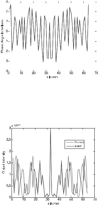
Figure 7.6. The output phase angle with the exactly computed and NFFA approximated diffraction integral.

where IExact and INFFA are the exact and NFFA intensities. Figure 7.6 shows the output phase angles for the exact method and the NFFA method almost perfectly overlapping each other.

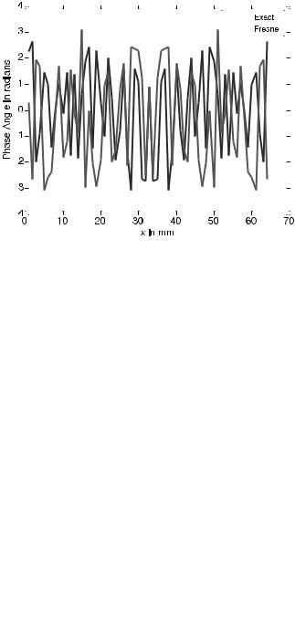
Figure 7.7 shows the output diffraction pattern intensity computed with the Fresnel approximation in comparison with the exact method. Figure 7.8 shows the

Figure 7.7. The output intensity with the Fresnel approximation in comparison with the exactly computed diffraction integral.

NUMERICAL EXAMPLES

105

Figure 7.8. The output phase angle with the Fresnel approximation in comparison with the output phase angle with the exactly computed diffraction integral.

output phase angle computed with the Fresnel approximation in comparison with the exact method. It is observed that the errors with the Fresnel approximation in the geometry considered are nonnegligible.

In the next set of experiments, 3-D results are discussed. Figure 7.9 shows the input square aperture used in the simulations. Two sets of parameters were used. In the first set, the parameters are as follows:

Z ¼ 50 mm; DI ðinput square aperture sideÞ¼ 0:2 mm; N ¼ 512; l ¼ 0:6328 m

Figure 7.9. The input square aperture used in simulations.

106	WIDE-ANGLE NEAR AND FAR FIELD APPROXIMATIONS

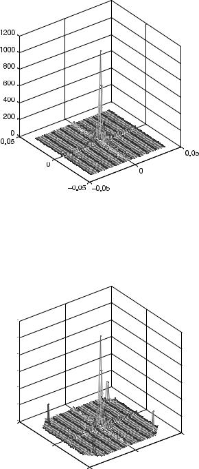
Figure 7.10. The output diffraction amplitude computed with the NFFA.

With the FFT conditions, the output plane aperture size becomes 0.081 mm on a side with these parameters. Figure 7.10 shows the 3-D plot of the output diffraction amplitude computed with the NFFA. Figure 7.11 shows the corresponding 3-D plot of the output diffraction amplitude computed with the Fresnel approximation.

1200

1000

800

600

400

200

0

0.05

0.05

0

0

–0.05 –0.05

Figure 7.11. The output diffraction amplitude computed with the Fresnel approximation.

NUMERICAL EXAMPLES

107

250

200

150

100

50

0

0.05

0.05

0

0

–0.05 –0.05

Figure 7.12. The error in diffraction amplitude (absolute difference between Figs. 7.11 and 7.12).

Figure 7.12 shows the error in diffraction amplitude (absolute difference between Figures 7.10 and 7.11). It is observed that the Fresnel approximation makes nonnegligible error in amplitude in certain parts of the observation plane in this geometry.

The second set of parameters was chosen as follows:

z ¼ 100 mm; DI ðinput square aperture sideÞ ¼ 2 mm; N ¼ 512; l ¼ 0:6328 m

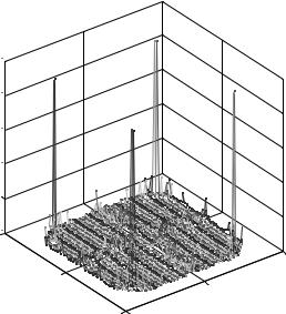
With the FFT conditions, the output plane aperture size becomes 16.2 mm on a side with these parameters. Figure 7.13 shows the 3-D plot of the output diffraction amplitude computed with the NFFA. Figure 7.14 shows the corresponding 3-D plot of the output diffraction amplitude computed with the Fresnel approximation. Figure 7.15 shows the error in diffraction amplitude (absolute difference between Figures 7.13 and 7.14). It is observed that the nonnegligible error in amplitude due to the Fresnel approximation in certain parts of the observation plane is less serious in this geometry because z is larger and the output size is smaller.

The final set of experiments was done with the checkerboard image of Figure 16 as the desired output amplitude diffraction pattern. The parameters of the experiments were as follows:

z ¼ 80 mm; DI ðinput square aperture sideÞ ¼ 0:8 mm; N ¼ 256; l ¼ 0:6328 m

With the FFT conditions, the output plane aperture size becomes 16.2 mm on a side with these parameters. The input diffraction pattern was computed in two ways. The