Ersoy O.K. Diffraction, Fourier optics, and imaging (Wiley, 2006)(ISBN 0471238163)(427s) PEo

138 FOURIER TRANSFORMS AND IMAGING WITH COHERENT OPTICAL SYSTEMS

Thus, the wave field at the focal plane of the lens is the 2-D Fourier transform of the wave field at z ¼ f if the effect of P(x,y) is neglected.

The limitation imposed by the finite lens aperture is called vignetting and can be avoided by choosing d1 small. To include the effect of the finite lens aperture, geometrical optics approximation can be used [Goodman]. With this approach, the initial wave field is approximated such that the finite pupil function at the lens equals

Pðx1 þ ðd1=f Þxf þ ðd1=f Þyf Þ. Then, Aðfx; fy; d1Þ with fx ¼ xf =lf and fy ¼ yf =lf is computed with respect to this pupil function. The wave field at z ¼ f becomes

Uðxf ; yf ; f Þ ¼ ej2f ð1 f Þðxf þyf Þ		ðð	Uðx; y; d1ÞP x þ	f1 xf ; y þ y1 yf e j l f ðxxf þyyf Þdxdy
	k d1 2 2	1		d	d	2p
		1				ð9:3-7Þ

9.3.3Wave Field to the Right of the Lens

The third possibility is to consider the initial wave field behind the lens, a distance d from the focal plane of the lens. This is the case when the lens is illuminated with a plane perpendicular wave field, and an object transparency is located at z ¼ f d as shown in Figure 9.4.

By geometrical optics, the amplitude of the spherical wave at this plane is proportional to f=d and can be neglected as constant. If ðx2; y2; f dÞ indicates a point on this plane, the equivalent pupil function on the object plane is Pðx2ðf =dÞ; y2ðf =dÞÞ due to the converging spherical wave. If Uðx2; y2; f dÞ is the wave field due to the object transparency, the total wave field at the object plane is given by

		k	2	2		f		f
U0	ðx2; y2; f dÞ ¼ e j	2d	ðx2	þy2	ÞP x2		; y2		Uðx2; y2; f dÞ	ð9:3-8Þ
						d		d

Let A0ðfx; fy; f dÞ be the angular spectrum of U0ðx2; y2; f dÞ. Provided that the Fresnel approximation is valid for the distance d, the angular spectrum of the wave field at the focal plane is given by

Aðxf ; yf ; f Þ ¼ A0ð fx; fy; f dÞe j									k	ðxf2þyf2Þ	ð9:3-9Þ
									2d

Figure 9.4. The geometry for the input to the right of the lens.

IMAGE FORMATION AS 2-D LINEAR FILTERING					139

Figure 9.5. The geometry used for image formation.

where constant terms are neglected fx and fy are xf =ld and yf =ld. With this geometry, the scale of the Fourier transform can be varied by adjusting d. The size of the transform is made smaller by decreasing d. In optical spatial filtering, this is a useful feature because the size of the Fourier transform must be the same as the size of the spatial filter located at the focal plane [Goodman].

9.4IMAGE FORMATION AS 2-D LINEAR FILTERING

Lenses are generally known as imaging devices. Imaging by a positive, aberrationfree thin lens in the presence of monochromatic waves is discussed below.

Consider Figure 9.5 in which transparent object is placed on plane z ¼ d1, and illuminated by a wave so that the wave field is Uðx1; y1; d1Þ on this plane.

The wave field Uðx0; y0; d0Þ on the plane z ¼ d0 is to be determined. Then, under what conditions an image is formed is discussed.

Since wave propagation is a linear phenomenon, the fields at ðx0; y0; d0Þ and ðx; y; d1Þ can always be related by a superposition integral:

Uðx0; y0; d0Þ ¼	ðð	hðx0; y0; x1; y1ÞUðx1; y1; d1Þdx1dy1	ð9:4-1Þ
	1
	1

where hðx0; y0; x1; y1Þ is the impulse response of the system. In order to find h, Uðx; y; d1Þ will be assumed to be a delta function at ðx1; y1; d1Þ. This is physically equivalent to a spherical wave originating at this point.

We will assume that the lens at z ¼ 0 has positive focal length f. All the constant terms due to wave propagation will be neglected. The field incident on the lens within the paraxial approximation is given by

	k		2	2
Uðx; y; 0Þ ¼ e j		ððx x1	Þ þðy y1	Þ Þ	ð9:4-2Þ
	2d1

The field after the lens is given by

U0ðx; y; 0Þ ¼ Uðx; y; 0ÞPðx; yÞe j	k	ðx2þy2Þ	ð9:4-3Þ
	2f

140 FOURIER TRANSFORMS AND IMAGING WITH COHERENT OPTICAL SYSTEMS

The Fresnel diffraction formula, Eq (5.2-13), yields

Uðx0; y0; d0Þ ¼ hðx0; y0; x1; y1Þ

¼	ðð	U0ðx; y; 0Þej 2dk0ððx0 xÞ2þðy0 yÞ2Þ dxdy			ð9:4-4Þ
	1
	1

In practical imaging applications, the final image is detected by a detector system that is sensitive to intensity only. Consequently, the phase terms of the form ejy can be neglected if they are independent of the integral in Eq. (9.4-4). Then, Eq. (9.4-4) can be simplified to

hðx0; y0; x1; y1Þ ¼

ðð

Pðx; yÞe j 2 ðx

þy

Þe jk d0

þd1

xþ d0

þd1 y dxdy

ð9:4-5Þ

1

kD 2

2

x0

x1

y0

y1

1

where

1		1		1		ð9:4-6Þ
D ¼		þ
	d1		d0		f

Consider the case when D is equal to zero. In this case, Eq. (8.4-5) becomes

hðx0; y0; x1; y1Þ ¼	ðð	Pðx; yÞe jl2dp0 ½ðx0þMx1Þxþðy0þMy1Þy&dxdy
	1
	1

where

M ¼ d0 d1

If P(x,y) is neglected, Eq. (8.4-7) is the same as

ðð1

hðx0; y0; x1; y1Þ ¼ e j2p½ðx1þxM0Þx0þðy1þyM0Þy0&dx0dy0

1

where x0 ¼ x=ld0 and y0 ¼ y=ld0, and a constant term is dropped. Equation (9.4-9) is the same as

	x0			y0
hðx0; y0; x1; y1Þ ¼ d x1 þ		; y1	þ
	M			M

Using this result in Eq. (9.4-1) gives

Uðx0; y0; d0Þ ¼ U x0 ; y0 ; d1 M M

ð9:4-7Þ

ð9:4-8Þ

ð9:4-9Þ

ð9:4-10Þ

ð9:4-11Þ

IMAGE FORMATION AS 2-D LINEAR FILTERING

141

We conclude that Uðx0; y0; d0Þ is the magnified and inverted image of the field at z ¼ d1, and M is the magnification when D given by Eq. (9.4-6) equals zero. Then, d0 and d1 are related by

1	1		1
	¼				ð9:4-12Þ
d0		f		d1

This relation is known as the lens law.

9.4.1The Effect of Finite Lens Aperture

Above the effect of the finite size pupil function P(x,y) was neglected. Letting

		x10 ¼ Mx1			ð9:4-13Þ
		y10 ¼ My1			ð9:4-14Þ
Equation (9.4-7) can be written as
		1
hðx0; y0; x10 ; y10 Þ ¼ ðð Pðld0x; ld0yÞe j2p½ðx0 x10 Þxþðy0 y10 Þy&dxdy					ð	9:4-15	Þ
		1
		¼ hðx0 x10 ; y0 y10 Þ
Then, Eq. (8.4-1) can be written as
Uðx0; y0	; d0	Þ ¼ ðð hðx0 x10 ; y0 y10	ÞUðx10	; y10 ; d1Þdx10 dy10	ð9:4-16Þ
		1
		1

where a constant term is again dropped. Equation (9.4-16) is a 2-D convolution:

Uðx0; y0; d0Þ ¼ hðx0; y0Þ U			x0		y0
				;		; d1		ð9:4-17Þ
			M		M
where Uðð x0=MÞ; ð y0=MÞ; d1Þ is the ideal image, and
hðx0; y0Þ ¼	ðð	Pðld0x; ld0yÞe j2pðx0xþy0yÞdxdy						ð9:4-18Þ
	1
	1

The impulse response is observed to be the 2-D FT of the scaled pupil function of the lens. The final image is the convolution of the perfect image with the system

142 FOURIER TRANSFORMS AND IMAGING WITH COHERENT OPTICAL SYSTEMS

impulse response. This smoothing operation can strongly attenuate the fine details of the image.

In a more general imaging system with many lenses, Eqs. (9.4-17) and (9.4-18) remain valid provided that P(.,.) denotes the finite equivalent exit pupil of the system, and the system is diffraction limited [Goodman]. An optical system is diffraction limited if a diverging spherical wave incident on the entrance pupil is mapped into a converging spherical wave at the exit pupil.

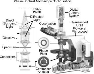
9.5PHASE CONTRAST MICROSCOPY

In this and the next section, the theory discussed in the previous sections is illustrated with two advanced imaging techniques. Phase contrast microscopy is a technique to generate high contrast images of transparent objects, such as living cells in cultures, thin tissue slices, microorganisms, lithographic patterns, fibers and the like. This is achieved by converting small phase changes in to amplitude changes, which can then be viewed in high contrast. In this process, the specimen being viewed is not negatively perturbed.

The image of an industrial phase contrast microscope is shown in Figure 9.6. When light passes through a transparent object, its phase is modified at each

point. Hence, the transmission function of the specimen with coherent illumination can be written as

tðx; yÞ ¼ e jðy0þyðx;yÞÞ

ð9:5-1Þ

where y0 is the average phase, and the phase shift yðx; yÞ is considerably less than

Figure 9.6. The schematic of an industrial phase contrast microscope [Nikon].

PHASE CONTRAST MICROSCOPY	143
2p. Hence, tðx; yÞ can be approximated as
tðx; yÞ ¼ e jy0 ½1 þ jyðx; yÞ&	ð9:5-2Þ

where the last factor is the first two terms of the Taylor series expansion of e jyðx;yÞ.

A microscope is sensitive to the intensity of light that can be written as
Iðx; yÞ ¼ j1 þ jyðx; yÞj2 1	ð9:5-3Þ

Hence, no image is observable. We note that Eq. (9.5-3) is true because the first term of unity due to undiffracted light is in phase quadrature with jyðx; yÞ generated by the diffracted light. In order to circumvent this problem, a phase plate yielding p=2 or 3p=2 phase shift with the undiffracted light can be used. This is usually achieved by using a glass substrate with a transparent dielectric dot giving p=2 or 3p=2 phase shift, typically by controlling thickness at the focal point of the imaging system. The undiffracted light passes through the focal point whereas the diffracted light from the specimen is spread away from the focal point since it has high spatial frequencies. On the imaging plane, the intensity can now be written as

Iðx; yÞ ¼ ejp=2 þ jyðx; yÞ 2 1 þ 2yðx; yÞ	ð9:5-4Þ
with p=2 phase shift, and
Iðx; yÞ ¼ ej3p=2 þ jyðx; yÞ 2 1 2yðx; yÞ	ð9:5-5Þ

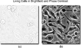
with 3p=2 phase shift. Equations (9.5-4) and (9.5-5) are referred to as positive and negative phase contrast, respectively. In either case, the phase variation yðx; yÞ is observable as an image since it is converted into intensity. An example of imaging with phase contrast microscope in comparison to a regular microscope is shown in Figure 9.7.

Figure 9.7. (a) Image of a specimen with a regular microscope, (b) image of the same specimen with a phase contrast microscope [Nikon].

144 FOURIER TRANSFORMS AND IMAGING WITH COHERENT OPTICAL SYSTEMS

It is possible to further improve the method by designing more complex phase plates. For example, contrast can be modulated by varying the properties of the phase plate such as absorption, refractive index, and thickness. Apodized phase contrast objectives have also been utilized.

9.6SCANNING CONFOCAL MICROSCOPY

The conventional microscope is a device which images the entire object field simultaneously. In scanning microscopy, an image of only one object point is generated at a time. This requires scanning the object to generate an image of the entire field. A diagram of a reflection mode scanning optical microscope is shown in Figure 9.8. Such a system can also be operated in the transmission mode. Modern systems feed the image information to a computer system which allows digital postprocessing and image processing.

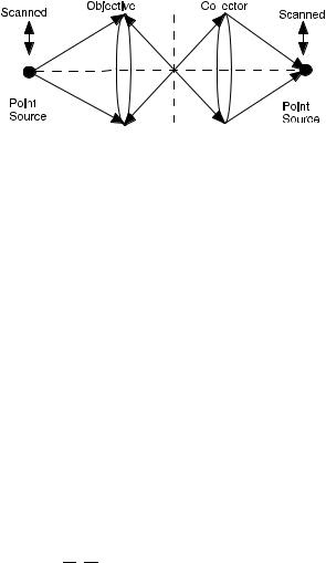
In scanning confocal microscopy, light from a point source probes a very small area of the object, and another point detector ensures that only light from the same object area is detected. A particular configuration of a scanning confocal microscope is shown in Figure 9.8 [Wilson, 1990]. In this system, the image is generated by scanning both the source and the detector in synchronism. Another configuration is shown in Figure 9.9. In this mode, the confocal microscope has excellent depth discrimination property (Figure 9.10). Using this property, parallel sections of a thick translucent object can be imaged with high resolution.

9.6.1Image Formation

Equation (9.4-16) can be written as

	1	1
	1 1
Uðx0; y0Þ ¼	ð ð		h x1 þ	x0	; y1	þ	y0	Uðx1; y1Þdx1dy1	ð9:6-1Þ
				M			M

where d0 and d1 are dropped from the input output complex amplitudes, to be understood from the context. The impulse response function given by Eq. (9.4-18)

X-Y

Laser

Scanning

Object

Detector		Display

Figure 9.8. Schematic diagram of a reflection mode scanning confocal microscope.

SCANNING CONFOCAL MICROSCOPY		145

Figure 9.9. A confocal optical microscope system.

can be written as

	1	1
hðx; yÞ ¼	ð	ð	Pðld0x1; ld0y1Þe 2pjðx1xþy1yÞdx1dy1	ð9:6-2Þ
	1 1

where Pðx1; y1Þ is the pupil function of the lens system.

In confocal microscopy, since one object point is imaged at a time, Uðx1; y1Þ can be written as

Uðx1; y1Þ ¼ dðx1Þdyðx1Þ

ð9:6-3Þ

Hence,

	1	1
Uðx0; y0Þ ¼	ð ð		h x1 þ	x0	; y1	þ	y0		dðx1Þdyðx1Þdx1dy1
				M			M				Þ
	1 1								ð	9:6-4

¼ h x0 ; y0 M M

The intensity of the point image becomes

Iðx0; y0Þ ¼	h M		; M			ð9:6-5Þ
		x0		y0		2

Assuming a circularly symmetric pupil function of radius a, Pðx1; y1Þ can be written as

x	1;	y	1Þ ¼	P	ðrÞ ¼	1 r 1=2	9	:	6-6	Þ
ð						0 otherwise	ð

146 FOURIER TRANSFORMS AND IMAGING WITH COHERENT OPTICAL SYSTEMS

where

	¼ p		ð		Þ
r		x12 þ y12		9:6-7
		2a

PðrÞ is the cylinder function studied in Example 2.6. The impulse response function becomes the Hankel transform of PðrÞ, and is given by

p

hðx0; y0Þ ¼ hðr0Þ ¼

sombðr0Þ

ð9:6-8Þ

4

where

q

r0 ¼ x02 þ y02

ð9:6-9Þ

somb r

0Þ ¼

2J1ðpr0Þ

ð

9:6-10

Þ

pr0

ð

The intensity of the point image becomes

MJ1 pr0=M

2

ð

Þ

Iðx0; y0

Þ ¼

2r0

ð9:6-11Þ

In practice, there are typically two lenses used, as seen in Figure 9.9. They are called objective and collector lenses. Suppose that the two lenses have impulse response functions h1 and h2, respectively. By repeated application of Eq. (9.7-1), it can be shown that the image intensity can be written as

Iðx0; y0Þ ¼ jht Uðx1; y1Þj2	ð9:6-12Þ
where
ht ¼ h1h2	ð9:6-13Þ

If the lenses are equal, with impulse response h given by Eq. (9.7-7), the output intensity can be written as

		MJ1	pr0	=M			4
			ð		Þ
Iðx0; y0Þ ¼			2r0				ð9:6-14Þ

EXAMPLE 9.1 Determine the transfer function of the two-lens scanning confocal microscope.

Solution: Since ht ¼ h1h2, we have

Htðfx; fyÞ ¼ H1ðfx; fyÞ H2ðfx; fyÞ

OPERATOR ALGEBRA FOR COMPLEX OPTICAL SYSTEMS

147

where, for two equal lenses,

H1ðfx; fyÞ ¼ H2ðfx; fyÞ ¼ Pðld0x1; ld0y1Þ

If the pupil function P is circularly symmetric, Htðfx; fyÞ is also symmetric, and can be written as

Htðfx; fyÞ ¼ HtðrÞ

where

q r ¼ fx2 þ fy2

Hence,

HtðrÞ ¼ H1ðrÞ H2ðrÞ

It can be shown that this convolution is given by
		"cos 1							r				#
	2						r			r		2
				r
HtðrÞ ¼	p			2				2	1	2

where

(

1 0 r 1

PðrÞ ¼

0otherwise

9.7OPERATOR ALGEBRA FOR COMPLEX OPTICAL SYSTEMS

The results derived in Sections 9.1–9.5 can be combined together in an operator algebra to analyze complex optical systems with coherent illumination [Goodman]. For simple results to be obtained, it is necessary to assume that the results are valid within the paraxial approximations involved in Fresnel diffraction and geometrical optics.

An operator algebra is discussed below in which the apertures are assumed to be separable in rectangular coordinates so that 2-D systems are discussed in terms of 1-D systems.

The operators involve fundamental operations that occur within a complex optical system. If U(x) is the current field, OðuÞ½U1ðxÞ& will denote the transformation