Ersoy O.K. Diffraction, Fourier optics, and imaging (Wiley, 2006)(ISBN 0471238163)(427s) PEo

148 FOURIER TRANSFORMS AND IMAGING WITH COHERENT OPTICAL SYSTEMS

of U1ðxÞ by the operator O(u) characterized by a variable u. Below the most important operators are described.

1. Fourier transform

					1
		U2ðvÞ ¼ FðvÞ½U1ðxÞ& ¼			ð	U1ðxÞe j2pvxdx			ð9:7-1Þ
					1
where n denotes frequency.
2. Free-space propagation
				1
			1	ð			k	2
U2	ðx2	Þ ¼ PðzÞ½U1ðx1	Þ& ¼ pjlz		U1	ðx1Þe j	2z	ðx2 x1Þ dx1	ð9:7-2Þ
				1

where k ¼ 2p=l, l is the wavelength, and z is the distance of propagation.

For a distance of propagation closer than the Fresnel region, the angular spectrum method can be used instead of Fresnel diffraction.

3.	Scaling by a constant			ðxÞ& ¼ pj j
	2ð	x	Þ ¼ SðaÞ½U1		U	1ð	ax	Þ	ð :	7-3	Þ
	U			a					9
	where a is a scaling constant.
4.	Multiplication by a quadratic phase factor
	U2ðxÞ ¼ QðbÞ½U1ðxÞ& ¼ e j 2k bx2 U1ðxÞ								ð9:7-4Þ
	where b is the parameter controlling the quadratic phase factor.

Each of these operators has an inverse. They are shown in Table 9.1.

In order to use the operator algebra effectively, it is necessary to show how two successive operations are related. These relationships are summarized in Table 9.2.

In this table, each element, say, E equals the successive operations with the row operator R(v1) followed by the column operator C(v2):

	E ¼ Cðv2ÞRðv1Þ					ð9:7-5Þ
Table 9.1. Inverse operators.
	FðnÞ	PðzÞ	SðaÞ			QðbÞ
			1
Inverse Operator	Fð nÞ	Pð zÞ	S			Qð bÞ
				a

OPERATOR ALGEBRA FOR COMPLEX OPTICAL SYSTEMS

149

Table 9.2. Operators and their algebra.

FðvÞ

PðzÞ

SðaÞ

QðbÞ

1

b

FðvÞ

Sð 1Þ

Qð lz2ÞFðvÞ

S

FðvÞ

P

FðvÞ

a

l2

1

1

Q"

þ z

#

b

P z

F v Q 2z

Pðz2ÞPðz1Þ

S a P a2

h

1

i

ð Þ

ð Þ ð l Þ

¼ Pðz1 þ z2Þ

ð Þ ð z Þ

1

S ð1 þ bzÞ

Phðz þ bÞ i

1

1

z

¼ ð

þ

Þ

S a

S a1

SðaÞ

FðvÞS

a

P

a2

SðaÞ

ð

2Þ Sð a1Þ

a2

Qða2bÞSðaÞ

b

P½ðz 1 þ bÞ 1&

b

Q

b2

Q b1

QðbÞ

FðvÞP

Sð1 þ1bzÞ 1

SðaÞQ

ð

ÞQðb1 Þ

l2

a2

b2

Þ

Q½ðb þ zÞ &

¼ ð

þ

In addition, the following relations are often used to simplify results:

1

1

1

PðzÞ ¼ Q

S

FðvÞQ

ð9:7-6Þ

z

lz

z

1

1

S

FðvÞ ¼ Pðf ÞQ

Pðf Þ

ð9:7-7Þ

lf

f

Equation (9.7-6) corresponds to Fresnel diffraction. Equation (9.7-7) shows that the fields at the front and back focal planes of a lens are related by a scaled Fourier transform.

EXAMPLE 9.2 (a) Simplify the following operator equation:

1

1

1

O ¼ Q

Pðf ÞQ

Pðf ÞQ

Pðf Þ

f

f

f

(b) Which optical system does this operator correspond to?

(c) Determine the final field Uend in terms of the initial field U1.

Solution: (a) The first three operators on the right hand side correspond to S

1

lf

1

1

1

S

using

FðvÞ by Eq. (9.7-7). Next P(f) is replaced

lf Fðv2

ÞQ

by

by Q f

f

Eq. (9.7-6). We get

1 1

O ¼ S lf Fðv2ÞS lf Fðv1Þ

(b) This operator corresponds to the optical system shown in Figure 9.10.

150 FOURIER TRANSFORMS AND IMAGING WITH COHERENT OPTICAL SYSTEMS

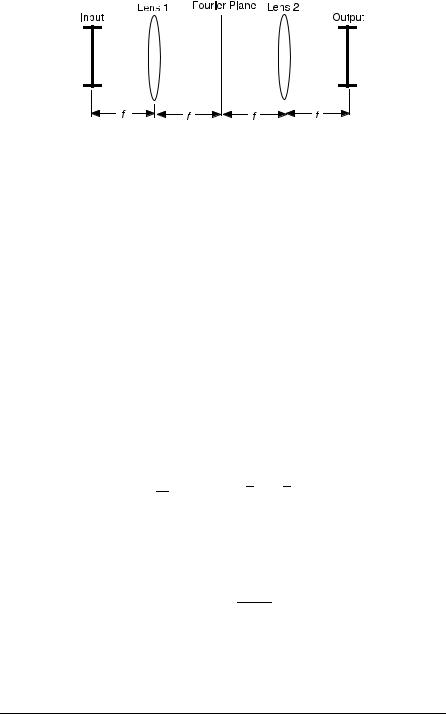
Figure 9.10. Final optical system for Example 9.2.

(c) Let us follow up each operator as an integral equation:

				1
	U2ðn1Þ ¼ Fðn1Þ½U1ðxÞ& ¼			ð	U1ðxÞe j2pn1xdx
	1
	U3ðn1Þ ¼ S		½U2ðn1Þ& ¼ p1lf			1
		1				ð U1ðxÞe j2p	n1		xdx
							lf
		lf
				1		1
	U4ðn2Þ ¼ Fðn2Þ½U3ðn1Þ& ¼			ð	U3ðn1Þe j2pn2n1 dr1
				1
	U5ðn2Þ ¼ S l1f ½U4ðn2Þ& ¼ p1lf					1
						ð U3ðr1Þe j2pnl2f n1 dn1
						1

Using the integral equation for U3ðn1Þ, the last equation is written as

ð1ð

U5ðn2Þ ¼ 1 U1ðxÞe j2pnl1f xe j2pnl2f r1 dxdv1

lf

		1
1		1			1		xþv2
		1		4 1				5
¼	lf	ð	U1ðxÞdx2 ð e j2pð				lf Þv1 dv13
		1			x þ v2
	1	ð	U	x		dx
¼ lf					lf
			1	ð Þd
		1

1ð

¼U1ðxÞdðx þ n2Þdx

1

¼ U1ð n2Þ

OPERATOR ALGEBRA FOR COMPLEX OPTICAL SYSTEMS

151

EXAMPLE 9.3 Show that the optical system shown below results in a Fourier transform in which the spatial frequency can be adjusted by changing z.

Solution: The operator O relating the output to the input is given by

O ¼ Pðz2ÞQ

1

PðzÞQ

1

f

z1 z

1

1

1

1

By using the lens law, namely, f

¼

þ

, Q f can be written as

z1

z2

1

1

1

Q

¼ Q

f

z1

z2

From Table 9.2, we use the following relations:

ð9:7-8Þ

ð9:7-9Þ

P

z2

Q

1 1

Q

z1 þ z2

S

z1

P

z1

9:7-10

Þ

z1 z2

¼

z22

ð

Þ

ð

Þ

ð

z2

1

z1

1

1

Pðz z1Þ ¼ Q

S

Q

S

FðrÞ ð9:7-11Þ

z z1

z2

z z1

lðz z1Þ

Substituting the results in Eqs. (9.7-9), (9.7-10), and (9.7-11) in Eq. (9.7-1) yields

O

¼

Q

z1 þ z2

S

z1

Q

1

S

1

F r

Þ

z22

z2 z

z1

lðz z1Þ

ð

Using the fact that

b

QðbÞSðaÞ ¼ SðaÞQ

a2

from Table 9.2 results in

z2

z2 z z1

¼

z22

S

z1

Q

1

Q

z1

þ z2

S

z1

152 FOURIER TRANSFORMS AND IMAGING WITH COHERENT OPTICAL SYSTEMS

This yields

O

¼

Q

z1 þ z2

Q

z1 þ z2

S

z1

S

1

F r

z22

z12

z2 lðz z2Þ

ð Þ

Combining successive Q as well as S operations results in

O

¼

Q

ðz1 þ z2Þz z1z2

S

z1

F r

Þ

z1

z

z22

ð

z

z1

Þ

lz2

ð

ð

Þ

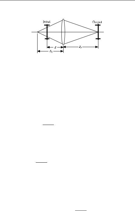
As an integral equation, O corresponds to

jkðz1þz2Þz z1z2x2

1

2pz1x0

U2ðx2Þ ¼ e 2

z2ðz1 zÞ

0

ð

U1ðxÞe j

xdx

lz2ðz1 zÞ

2

1

By varying z, the spatial frequency

z1x0

can be adjusted.

z2

ðz1 zÞ

10

Imaging with Quasi-Monochromatic Waves

10.1INTRODUCTION

In previous chapters, wave propagation and imaging with coherent and monochromatic wave fields were discussed. In this chapter, this is extended to wave propagation and imaging with quasi-monochromatic coherent or incoherent wave fields.

Monochromatic wave fields have a single temporal frequency f. Nonmonochromatic wave fields have many temporal frequencies. Quasi-monochromatic wave fields have a temporal frequency spread f , which is much less than the average temporal frequency fc. In practical imaging applications, wave fields can usually be assumed to be quasi-monochromatic.

This chapter consists of 10 sections. The first few sections lay the groundwork for the theory that is pertinent for analyzing quasi-monochromatic waves. Section 10.2 introduces the Hilbert transform that is closely related to the Fourier transform. Its main property is swapping the cosine and sine frequency components. It is a tool that is needed to define the analytic signal described in Section 10.3. The analytic signal is complex, with its real part equal to a real signal and its imaginary part equal to the Hilbert transform of the same real signal. In addition to its use in analyzing quasi-monochromatic waves, it is commonly used in analyzing single-sideband modulation in communications.

Section 10.4 shows how to represent a quasi-monochromatic wave in terms of an analytic signal. The meanings of quasi-monochromatic, coherent, and incoherent waves are more closely examined in Section 10.5 with spatial coherence and time coherence concepts.

The theory developed up to this point for simple optical systems is generalized to more complex imaging systems in Section 10.6. Imaging with quasi-monochromatic waves is the subject of Section 10.7. The difference between coherent imaging and incoherent imaging becomes clear in this section. A diffraction-limited imaging system is considered as a linear system in Section 10.8, and its linear system properties are derived for coherent and incoherent imaging. One of these properties is the optical transfer function. How it can be computed with a computer is the topic

Diffraction, Fourier Optics and Imaging, by Okan K. Ersoy

Copyright # 2007 John Wiley & Sons, Inc.

153

154	IMAGING WITH QUASI-MONOCHROMATIC WAVES

of Section 10.9. All imaging systems have aberrations. They are described in Section 10.10, especially in terms of Zernike polynomials.

10.2HILBERT TRANSFORM

The Hilbert transform and the analytic signal discussed in Section 10.3 are useful in characterizing quasi-monochromatic fields and image formation. They are also useful in a number of other applications such as single sideband modulation in communications [Ziemer and Tranter, 2002]. The Hilbert transform of a real signal vðtÞ is defined as

				1		uðtÞ
	v t		1	ð			d	t		10:2-1
		Þ ¼ p			t t				ð		Þ
	ð
				1

This is the convolution of uðtÞ with the function 1=pt.

Using the convolution theorem, Eq. (10.2-1) in the Fourier domain can be written

as
Vð f Þ ¼ Uð f ÞHð f Þ				ð10:2-2Þ
where Hð f Þ is the FT of 1=pt, given by
Hð f Þ ¼ j sgnð f Þ				ð10:2-3Þ
The sgn function sgnð f Þ is defined by
	8	1	f > 0
	>
	>
sgnð f Þ ¼	<	0	f ¼ 0	ð10:2-4Þ
	>	1	f < 0
	:
	>

Using Parseval’s theorem and Eq. (10.2-2), it is observed that the energy of vðtÞ is equal to the energy of uðtÞ:

1		1
ð	v2ðtÞdt ¼	ð	u2ðtÞdt	ð10:2-5Þ
1		1

Equation (10.2-3) shows that the Hilbert transform shifts the phase of the spectral components by p=2. That is why it is also called the quadrature filter.

HILBERT TRANSFORM

155

The inverse Hilbert transform can be shown to be

				1		vðtÞ
	u t		1	ð			d	t	ð	10:2-6	Þ
		Þ ¼ p			t t
	ð
				1

The integral involved in the Hilbert transform is an improper integral, which is actually an abbreviation of the following:

1

u t

t e

u t

1

u t

lim

t

2

t ð Þ dt þ

t

ð Þ dt3

ð10:2-7Þ

ð

ð Þ dt ¼ e 0

ð

t

!

t

ð

t

1

4 1

tþe

5

It can also be written as

1

uðtÞ

1

uðt þ tÞ

ð

d

t ¼

ð

d

t

ð

10:2-8

Þ

t t

t

1

1

EXAMPLE 10.1 Find the Hilbert transform of uðtÞ ¼ cosð2pf0t þ fð f0ÞÞ.

Solution:

1

1 cos 2pf0

t

1

1 cos 2

f0 t

vðtÞ ¼

ð

ð ð

ÞÞ

dt ¼

ð

ð

p ð

þ tÞÞ

dt

p

t t

p

t

1

1

ð

1

1

cos 2

f

0

t

f

cos 2

f

f

sin 2

f

t

f

sin

2f

¼

ð

p

þ fð

ÞÞ

ð

p 0t þ fð

0ÞÞ

ð

p 0

þ fð 0

ÞÞ

ð

0tÞ

dt

p

1

t

t

The first term is odd in t and integrates to zero. Then,

1ð

vðtÞ ¼ sinð2pf0t þ fð f0ÞÞ sinð2pf0t þ fð f0ÞÞ dt ¼ sinð2pf0 p t

ð10:2-9Þ

t þ fð f0ÞÞ

1

ð10:2-10Þ

EXAMPLE 10.2 Show that a real signal uðtÞ and its Hilbert transform vðtÞ are orthogonal to each other.

156 IMAGING WITH QUASI-MONOCHROMATIC WAVES

Solution: Using Parseval’s theorem, we write

1

1

ð

uðtÞvðtÞdt ¼

ð

Uð f ÞV ð f Þdf

1

1

1

0

¼ j ð jUð f Þj2df j

ð

jUð f Þj2df ¼ 0

0

1

ð10:2-11Þ

Uðf Þ ¼ U1ð f Þ jU0ð f Þ

u1

ð

t

Þ ¼

1

ð

Þ þ

u

ð

Þ

1

2

u t

t

x y 0ðzÞ ¼

2 uðtÞ uð tÞ

u

t

ð 0; 0;

Þ

t2 t1

because Uð f Þ ¼ U ð f Þ.

EXAMPLE 10.3 The FT of uðtÞ can be written as

Uð f Þ ¼ U1ðf Þ jU0ð f Þ

where U1ð f Þ and U0ð f Þ are the cosine and sine parts of the FT of uðtÞ.

Show that U1ð f Þ and U0ð f Þ are a Hilbert transform pair when uðtÞ is a causal signal (uðtÞ equals zero for negative t).

Solution: The even and odd parts of uðtÞ can be written as

1

u1ðtÞ ¼ 2 ½uðtÞ þ uð tÞ&

1

u0ðtÞ ¼ 2 ½uðtÞ uð tÞ&

When uðtÞ is causal, it is straightforward to show that

u1ðtÞ ¼ u0ðtÞsgnðtÞ
		ð10:2-14Þ
u0ðtÞ ¼ u1ðtÞsgnðtÞ
Then,
	1
U1ð f Þ ¼	ð	u1ðtÞe j2pftdt
	1	ð10:2-15Þ
	1
¼	ð	u0ðtÞsgnðtÞe j2pftdt
	1

ANALYTIC SIGNAL

157

By the modulation property of the Fourier transform,

U1ð f Þ equals

1the

convolution of the FT of u0ðtÞ equal to jU0ð f Þ and the FT of sgn(t) equal to

:

jpf

1

U1ð f Þ ¼

ð

jU0ðvÞ

1

dv

ð10:2-16Þ

jpð f vÞ

1

Thus,

1

U0ðvÞ

U

f

1

ð

dv

ð

10:2-17

Þ

Þ ¼ p

1ð

f v

1

It can be similarly shown that

1

U1ðvÞ

U

f

1

ð

dv

ð

10:2-18

Þ

0

ð

Þ ¼ p

f v

1

Equations (10.2-17) and (10.2-18) are also called Kramers–Kro¨nig relations

in

electromagnetics.

10.3ANALYTIC SIGNAL

The analytic signal is useful in understanding the properties of narrowband waveforms, wave propagation, and image formation. It is defined as

sðtÞ ¼ uðtÞ þ jvðtÞ

ð10:3-1Þ

where uðtÞ is a real signal, and vðtÞ is its Hilbert transform. Thus, the analytic signal is a means of converting a real signal to a complex signal. Taking the FT of both sides of Eq. (1.18.1) gives

Sð f Þ ¼ Uð f Þ þ jVð f Þ

ð10:3-2Þ

As Vð f Þ ¼ j sgnð f ÞUð f Þ, we get

8

Uð f Þ

f ¼ 0

S

ð

f

Þ ¼

2U

ð

f

Þ

f > 0

ð

10:3-3

Þ

>

<

>

0

f < 0

:

Hence, the analytic signal is given by

1

ð

ð10:3-4Þ

sðtÞ ¼ 2 Uð f Þej2pftdf

0