ELECTRICAL CONDUCTIVITY OF WEAKLY NONIDEAL PLASMA 255

ohm cm

.

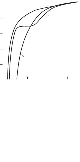
Fig. 6.2. Electrical conductivity of plasma of three di erent compositions at a pressure of

1atm.

6.2Electrical conductivity of weakly nonideal plasma

In a weakly ionized plasma, the nonideality is caused by charged particle–atom interactions. The nonideality may a ect both the concentration of free electrons and their mobility. The e ect of nonideality on ne was discussed earlier in Section 4.3. This e ect is due to the reduction of the ionization potential and the emergence of cluster ions. In moderately dense vapors the former e ect is still small (∆I T ), however, the inclusion of molecular ions brings about an appreciable variation of ne. This region of the ρ −T diagram for cesium in Fig. 6.1 is marked as VI.

On substituting in Eq. (6.1) the expression (4.32) or (4.49) for ne, derived with due regard for cluster ions, one can observe how the emergence of cluster ions a ects the density dependence of the electrical conductivity. At high temperatures and low concentrations, the scaling ne √na (see Eq. 6.2) is valid, and

the electrical conductivity decreases with an increase of density, σ n−a 1/2. With a decrease of temperature and increase of concentration, cluster ions emerge. If A+3 prevails among positive ions and A− among negative ions (the binding energy of A−2 is low), then it follows from Eqs.(4.32) and (6.5) that the electrical conductivity is independent of na. If the A+4 ion prevailed, the value of σ would increase with the growth of na as σ n1a/2.

Since the “ion–atom” interaction in plasmas of metal vapors is stronger than the “electron–atom” interaction, the nonideality parameter can be introduced as

Fig. 6.3.

256 ELECTRICAL CONDUCTIVITY OF PARTIALLY IONIZED PLASMA

ohm cm

Coe cient of electrical conductivity σ of sodium plasma at a pressure p ≈ 0.5ps: the points correspond to experiment (Morrow and Craggs 1973); the curves correspond to calculation (Khrapak 1979): 1 – eight–component composition of plasma; 2 – three–com- ponent composition.

the relation

γai = n+3 /n+2 = naK4/K3K5.

The condition γai = 1 defines the boundary separating the regions V and VI in Fig. 6.1. If γai > 1, then n+3 > n+2 . This means that one should expect the emergence of A+4 and maybe then A+m, where m 1.

The first experimental study, the results of which had pointed to the e ect of ionic complexes on electrical conductivity, was carried out by Morrow and Craggs (1973). The measurements in sodium vapors were performed at p ≈ 0.5ps (ps is the saturated vapor pressure), T = 1200–1500 K. The results of calculation, performed by Khrapak (1979) using the procedure described in Section 4.3, are in good agreement with experiment (see Fig. 6.3). In Fig. 2.11 the results of analogous calculations (Gogoleva et al. 1984) are compared with the measured values of the electrical conductivity of cesium vapors. A comparison of the calculation and measurement results points to their good agreement.

Figure 6.4 gives the isobars of the coe cient of electrical conductivity of sodium and lithium plasma, with the coe cient of electrical conductivity for cesium plasma being tabulated in Table 6.2. The pressure and temperature range

ELECTRICAL CONDUCTIVITY OF WEAKLY NONIDEAL PLASMA 257

ohm cm ohm cm

MPa

MPa

a

b

Fig. 6.4. Isobars of electrical conductivity of sodium (a) and lithium (b) plasma (Khrapak

1979).

covered by calculations is limited by the condition γai 1 in the case of low temperatures and high pressures and by the condition ln Λ 1 in the case of high temperatures. Therefore, the p > 1 MPa isobars are absent. Indeed, at p = 2 MPa, the description of the experimental isobar of the electrical conductivity of cesium vapor with the aid of analogous calculations is markedly poor. We speak of the portion of the isobar of electrical conductivity, shown in Fig. 2.9, which corresponds to high temperatures. An adequate description is attained (curve 2 in Fig. 2.9) only upon inclusion of density corrections to the electron mobility, which are discussed below.

As previously noted, the Lorentz formula for the electron mobility (Eq. 6.3) is derived assuming binary collisions, and hence is applicable under conditions when the characteristic radius of the interaction forces is much smaller than the electron free path. In other words a small number of particles must be present in the sphere of interaction on average, that is, the following inequality should be satisfied:

(4π/3)naq3/2 1.

(6.13)

At densities na = 1020 cm−3, the quantity (4π/3)naq3/2 in a cesium plasma reaches a value close to unity (q = 300−400πa20, see Table 6.1). Under conditions

258 ELECTRICAL CONDUCTIVITY OF PARTIALLY IONIZED PLASMA

when the inequality (6.13) is violated, one must allow for the collisions between three, four, and more particles.

This, however, does not mean that in a plasma of metal vapors the electron mobility becomes, with a rise in density, less than the mobility µ0 calculated for the same density from the Lorentz formula. It is not always the case that one can describe the electron–atom interaction as a scattering by a hard sphere with a radius of the order of √q. If the atomic polarizability is su ciently high, the “electron–atom” interaction is mainly a polarization one. The negative sign of the scattering length may serve as an indication of this. Dense vapors of metals fall under the category of precisely such strongly polarizable media. Therefore, their compaction may cause an increase of mobility instead of its decrease. This e ect is well known in the physics of dense fluids, the latter being referred to as “high mobility” fluids. A discussion of these e ects can be found in the paper by Atrazhev and Yakubov (1980).

As a result of interferences of potentials from neighboring and more remote particles, the total field of scatterers is smoothed. In describing this e ect, the

Table 6.2 Electrical conductivity of cesium plasma, ohm−1 m−1 (Gogoleva et al. 1984).

T , K	p = 10−4 MPa			10−3 MPa			10−2 MPa	10−1 MPa	1 MPa
1000	4.97 · 10−4			1.57 · 10−4			4.95 · 10−5	—		—
1200	2.71 · 10−2			8.56 · 10−3			2.70 · 10−3	8.42 · 10−4		—
1400	4.84 · 10−1			1.54 · 10−1			4.87 · 10−2	1.54 · 10−2		—
1600	4.19			1.37			4.37 · 10−1	1.40 · 10−1	5.11 · 10−2
1800	2.09 ·		101	7.38			2.43	7.89 · 10−1	2.94 · 10−1
2000	6.56	·	2	2.71	·	1	1	3.18	1.21	·	10−1
			101			101	9.54
2200	1.42 ·		102	7.23 ·		102	2.84 · 101	9.89 1	3.83
2400	2.36 ·		102	1.49 ·		102	6.78 · 102	2.53 · 101	1.00
2600	3.32 ·		102	2.51 ·		102	1.35 · 102	5.53 · 102		—
2800	4.23 ·		102	3.67 ·		102	2.31 · 102	1.06 · 10		—
3000	5.09 ·		102	4.86 ·		102	3.53 · 102	—		—
3200	5.87 ·		102	6.04 ·		102	4.92 · 102	—		—
3400	6.58 ·		102	7.10 ·		102	6.42 · 102	—		—
3600	7.20 ·		102	8.27 ·		102	7.98 · 102	—		—
3800	7.75 ·		102	9.28 ·		103	9.56 · 103	—		—
4000	8.27 ·		102	1.02 ·		103	1.11 · 103	—		—
4200	8.74 ·		102	1.10 ·		103	1.26 · 10	—		—
4400	9.21 ·		102	1.17 ·		103	—	—		—
4600	9.68 ·		103	1.24 ·		103	—	—		—
4800	1.02 ·		103	1.30 ·		103	—	—		—
5000	1.06 ·		10	1.36 ·		10	—	—		—

ELECTRICAL CONDUCTIVITY OF WEAKLY NONIDEAL PLASMA 259

following considerations are important. The potential of the “electron–isolated atom” interaction can be expressed as

V (r) =	2π 2	Lcδ(r) −	αe2		(6.14)
				.
	m		2(r2 + ra2)2

Here, the short–range component is written in the form of the Fermi pseudopotential (1.15). The quantity Lc is the length of electron scattering by the potential V (r). The polarization component in (6.14) features correct asymptotic behavior, α is the atomic polarizability and the cuto parameter ra corresponds to the size of the outer electron shell, i.e., the atomic radius. The amplitude of scattering, f (θ), and the length of scattering L by the potential (6.14) take the form

f (θ) = −L −	πα		θ			πα
		sin		,	L = Lc −		,	(6.15)
	2a0λ		2			4a0ra

where λ = (2mE)−1/2 is the wavelength of electron with energy E.

Equation (6.15) is valid for slow electrons while the following inequalities are

satisfied:

λ Lc, λ ra, λ2 α/a0.

An electron moving in a dense medium polarizes the latter. Internal fields occur, which reduce the electron–atom interaction. The polarization e ect can be readily included by introducing the dielectric permeability ε = 1 + (8π/3)αna and replacing the potential (6.14) by the potential of electron–atom interaction in the medium,

V (r) =	2π 2		αe2
		Lcδ(r) −		.
	m		2ε(r2 + ra2)2

If (8π/3)αna 1, the length of scattering in the medium is (Atrazhev and Yakubov 1980)

Lm = L +	4π2α2na	.	(6.16)
	3a0ra

This suggests that, if L < 0 (i.e., attraction prevails in the electron–atom interaction), |Lm| < |L|. In other words, the interaction weakens with an increase of density.

Atoms of alkali metals feature very high values of polarizability (α 100a30). In order to produce a qualitatively correct result one can write the approximate expression for the electron scattering cross–section in a medium as

qm(E) = q(E)(1 − ξ)2, ξ =	4π5/2α2na		,	(6.17)
	3a0ra
		q(E)

where the parameter ξ allows for the dielectric screening of the polarization interaction. Under experimental conditions (Alekseev et al. 1975), the value of the parameter ξ is of the order of 0.2. As a result, the correction to electron mobility, µ/µ0 = (1 − ξ)−2, is appreciable.

260 ELECTRICAL CONDUCTIVITY OF PARTIALLY IONIZED PLASMA

.

.

.
a	cm

Fig. 6.5. The measured values of µ/µ0 at T = 300 K as a function of atom density na

(Khrapak and Yakubov 1981).

In addition to the polarization e ect, a whole number of factors a ect the electron mobility. Let us discuss some of them. The interference e ect (Iakubov and Polishchuk 1982) occurs when the de Broglie electron wavelength λ becomes comparable with the electron free path (qna)−1. Then, two successive scattering events overlap. The emerging correction can be interpreted as a correction increasing the collision frequency νe = ν(1 + 2naqλ). As a result, the mobility decreases as compared with the ideal–gas case:

µ = µ0(1 −	√
		πnaqλ).

However, as the temperature increases, the interference e ect disappears because the thermal wavelength λ = (2mT )−1/2 decreases.

Therefore, as the density increases, the relative mobility may both decrease and increase. Figure 6.5 gives the results of measurements performed in di erent gases; see the list of references in Khrapak and Iakubov (1981). In polarizable gases, µ/µ0 > 1, and in poorly polarizable gases, µ/µ0 < 1. As follows from Fig. 6.5, the density e ects in mobility for atomic and molecular gases, for which q 10−15 cm2, occur at na 1021 cm−3. In the plasma of alkali metals, considerable deviations of from µ0 should occur at na 1019 cm−3.

As mentioned above, the values of the coe cient of electrical conductivity, which exceed the Spitzer values σSp, cannot be attained under standard conditions. This fact is due to the additivity of the frequencies ν and νi in the formula

ELECTRICAL CONDUCTIVITY OF WEAKLY NONIDEAL PLASMA 261

for electron mobility µ = (e/m)(ν + νi)−1. It should be borne in mind, however, that the additivity of ν and νi in a very dense plasma may be disturbed. For this, in passing over the Landau length e2/T , an electron must manage to repeatedly interact with many atoms, that is, the inequality e2qna/T 1 must be satisfied.

Under these conditions, in a first approximation, the electron–ion collisions have no e ect whatsoever on the mobility and may be ignored. Therefore, the values of σ in a dense medium are not restricted to Spitzer values.

Let us now treat the mobility in a medium of correlated scatterers. In a weakly ionized gas, the mobility may be strongly a ected by interatomic correlations. The square of the amplitude of electron scattering in the medium must be averaged with due regard for the correlation between atoms rather than over their chaotic distribution. As a result, the expression for the averaged collision frequency varies. This frequency contains the structure factor of the medium; see, for example, Kirzhnits et al. (1975). This situation is typical of liquid metals

and semiconductors.						j V (r−
R	Consider the electron scattering amplitude f (k) in the field U (r) =
	j) produced by atoms located at points Rj . In the Born
	f (k) = −(m/2π )2		exp(−ikr)[U(r) −		] dr,
				U

where k is the momentum transferred upon collision, and U is the mean field. The scattering probability is proportional to the square of amplitude f 2,

averaged over the distribution of scatterers,

f (k)2 =		2		Vk2		ΣΩN	×
	2πm			2		dR1 . . . dRN
				i j
										.
	× exp [−ik(Rj + Ri) + Ua/T ] − δ2(k)(na								)2		(6.18)
								V

Here, Vk is the Fourier component of the V (r) potential;

V =	V (r)dr, Ua = 2 m,n Va (Rm − Rn) ,
	1

where Va is the potential of interatomic interaction; N is the total number of gas atoms, N = naΩ; Ω is the system volume; and

Σ = Ω−N dR1 . . . dRN exp(−Ua/T )

is the partition function of the gas.

The term in curly brackets in (6.18), corresponding to i = j, is equal to N Vk2. This is a usual result of the kinetic theory of gases. With due regard for correlation, the terms corresponding to i =j are reduced to the emergence