The Physics of Coronory Blood Flow - M. Zamir

2.2 The “Lumped Model” Concept

37

we examine some of them subsequently, but the emphasis in this book is less on the models themselves than on the elements from which the models are constructed. The reason for this is that a model of the coronary circulation is only useful if it can be tested against some direct measurements. In fact, the model must be tailored to the type of measurements available, and as the nature and availablility of such measurements changes, so must the design and nature of the model to be used.

Our understanding of the dynamics of the coronary circulation is presently at its infancy. Indeed, in the clinical setting a purely static view of the system predominates, in which the concern is primarily with whether vessels are fully open or restricted by disease [127, 133, 73]. The reason for this viewpoint is not that the dynamics of the coronary circulation are thought unimportant in the clinical setting but that as yet we do not have a clear understanding or a clear model of these dynamics. The purpose of this book is to provide the student, researcher, or indeed clinician, with basic analytical and conceptual tools with which to explore and hopefully improve his or her understanding of the dynamics of the coronary circulation.

2.2 The “Lumped Model” Concept

The relation between pressure and flow in a tube depends on such properties of the tube as its diameter, length, and elasticity. It also depends on the form of the driving pressure, in particular whether the pressure is steady or pulsatile. The relation between pressure and flow in a vascular tree structure consisting of a large number of tube segments depends not only on all such factors in each tube segment but also on events at the junctions between tube segments and on how the properties of individual segments are distributed within the tree structure. The overwhelming complexity of this problem gives rise to the “lumped model” concept. Detailed analysis and results based on this concept are presented in subsequent chapters. Here we discuss only broadly the concept itself as a valid modelling strategy.

Essentially, in a lumped model the complex vascular structure of the coronary network is ignored and the network is replaced by a single tube having properties representative of the network as a whole. It is a variant of the more familiar “black box” concept, in which a complex system is enclosed by an imaginary box and only the relation between input and output from the box is examined to learn something about the characteristics of the system without delving into the complexity that produced these characteristics. In the coronary circulation the lumped model attempts to reproduce a relation between pressure and flow similar to that observed or measured in the physiological system but without going through the overwhelming task of determining how the relation unfolds through the complex structure of the coronary vascular network.

38 2 Modelling Preliminaries

Of particular interest is the relation between pressure and flow at input to the system and pressure and flow at output. The reason for this is that while some direct measurements of pressure and flow are possible at input to the system, usually at the left or right main coronary arteries, no such measurements are possible at output, that is at the capillary end of the system. The output end of the coronary circulation is of course of particular clinical interest because it represents the ultimate function of the system, namely the delivery of blood to cardiac tissue. But at this end of the system flow is divided into many millions of capillaries in which neither the velocity nor the number of capillaries can be determined with su cient accuracy to compute total output. A correct model of the system would thus provide a theoretical means of obtaining important information at output which is not available experimentally. However, the “correctness” of the model can ultimately be verified only by testing its results against some measurements from the physiological system. Thus, the modelling process becomes a highly intricate iterative process whereby the choice and values of model parameters are guided by a comparison of the results of the model with whatever direct measurements are available [110, 24, 115, 90, 98, 97].

Pressure and flow in the coronary circulation are highly pulsatile because of the pulsatile nature of the input driving pressure and because, in addition to this, much of the coronary vasculature is imbedded in cardiac muscle tissue and is subject to the e ects of cyclic contraction of the cardiac muscle, socalled “tissue-pressure e ects”. Thus, pressure and flow at both ends of the system are time-dependent in the sense that they have cyclic waveforms. The waveforms are not the same at both ends, however. At any point in time within the oscillatory cycle, total inflow into the coronary system is not usually equal to total outflow because of the so-called “capacitance” e ect. There is continuous change in the total volume of vascular lumen within the system during the oscillatory cycle. Therefore, some inflow may go towards “inflating” the system and will not contribute to outflow and, conversely, some outflow may be produced by “deflation” of the system rather than by direct inflow. While average flow must be the same at both ends of the system, that is, flow averaged over one or more cycles, a relation between average flow and average pressure does not feature the time-dependent characteristics of the system that actually contribute to that relation. Only events within the oscillatory cycle exhibit these characteristics, but the nature of these events is lost in the time-averaging process. For these reasons the main focus of lumped models has been on a time-dependent relation between pressure and flow, that is on the time course of that relation within the oscillatory cycle.

2.3 Flow in a Tube

At the core of almost every modelling scheme for coronary blood flow and for blood flow in general is the mechanics of flow in a tube. Indeed, the lumped

2.3 Flow in a Tube

39

model discussed in the previous section is based on the concept that flow through the complex vasculature of the coronary circulation can be replaced by flow in a single tube with “equivalent” properties. It is important, therefore, to outline the basic properties of flow in a single tube, which we do in this section. The validity of the basic premise of the lumped model concept, namely that flow in a complex system of vessels can be considered equivalent to flow in a single tube, can only be discussed in the context of each particular modelling scheme and is therefore deferred to subsequent chapters.

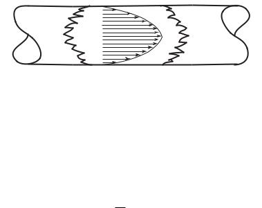
When fluid enters a tube, it does not simply slide along the tube as a bullet, because of a condition of “no-slip” that prevails at the tube wall [13, 34, 174, 71] whereby elements of fluid in contact with the tube wall become arrested there, forming a cylindrical layer of stationary fluid attached to the inner surface of the tube wall. As fluid progresses along the tube, the next layer of fluid adjacent to the first is slowed down by the stationary layer because of the viscosity of the fluid, and similarly, subsequent concentric layers of fluid that are further and further away from the wall are slowed down but to a lesser and lesser extent and are thus able to move more freely, fluid along the axis of the tube able to move the fastest (Fig. 2.3.1).

Fig. 2.3.1. Fully developed flow in a tube, commonly referred to as Poiseuille flow, is characterized by a parabolically shaped velocity profile, with zero velocity at the tube wall and maximum velocity along the tube axis.

Ultimately, at some distance downstream from the tube entrance, the flow becomes “fully developed” and is generally referred to as “Hagen-Poiseuille flow” after those who studied it first [168, 192, 174, 135], or more commonly as simply “Poiseuille flow”. Flow in this region is characterized by a parabolically shaped “velocity profile” along a diameter of the tube, with zero velocity at the tube wall and maximum velocity at the tube axis, and is given by [221]

u =	k	(r2 − a2)	(2.3.1)
	4μ

where μ is viscosity of the fluid, r is radial coordinate measured from the axis of the tube, a is the tube radius, and k is the pressure gradient driving the flow, which in Poiseuille flow is constant and equal to the pressure di erence Δp between any two points along the tube divided by the length of tube l between them, that is [221]

40	2 Modelling Preliminaries
	k =	dp	=	Δp		(2.3.2)
		dx			l

Here p is pressure and x is axial coordinate, positive in the direction of flow. The pressure di erence Δp is measured in the direction of flow, that is

Δp = p2 − p1

(2.3.3)

where p1, p2 are pressures at the upstream and downstream ends of the tube segment, respectively. Since p1 must be higher than p2 to produce flow in the positive x−direction, Δp is usually referred to as the “pressure drop” along the tube segment.

Eq. 2.3.1 indicates that in Poiseuille flow the flow rate q through the tube is given by

	a		−	kπa4
	q = 0	2πrudr =		8μ	(2.3.4)

Thus, average flow velocity u is given by

		=	q	=	−ka2	(2.3.5)
	u
			πa2		8μ

while maximum velocity uˆ occurs on the tube axis where r = 0 and from Eq. 2.3.1 is given by

	uˆ =	−ka2	(2.3.6)
		4μ

The two results show that maximum velocity in Poiseuille flow is twice the average velocity, that is

uˆ = 2		(2.3.7)
	u

As described earlier, Poiseuille flow is not established immediately on entry into the tube, but evolves over a length of tube le known as the “entry length”. Flow in that region of the tube is usually referred to as “developing flow” and an estimate of the entry length is given by [123, 174, 71]

le = 0.04NRd

(2.3.8)

where d is tube diameter and NR is the Reynolds number, defined by

	NR =	ρud			(2.3.9)
		μ

where ρ is fluid density.

When the lumped model is used to study flow in the coronary circulation, which means that coronary blood flow is being modelled by an equivalent flow

2.4 Fluid Viscosity: Resistance to Flow

41

in a single tube, the equivalent flow is invariably considered fully developed. This assumption is fairly di cult to deal with because it is at once both necessary and unjustified. The assumption is unjustified because the entry lengths in many millions of tube segments in the coronary circulation will be di erent and cannot be represented by an “equivalent” entry length in a single tube. Furthermore, the assumption is necessary because the problem of determining the entry length and examining the extent to which flow is fully developed in each of these millions of tube segments is intractable. It is in fact further complicated because flow is entering and leaving tube segments at di erent stages of development. As a result, the standard entry length analysis leading to the result in Eq. 2.3.8, based on the assumption that flow entering the tube is uniform, no longer applies [31]. The best that can be done is to evaluate the weight of the assumption of fully developed flow in each modelling scheme in context of the particular aspect of coronary circulation being studied.

If flow entering a tube is assumed to have a uniform velocity u, then a key di erence between the developing and fully developed regions of the flow is that in the developing region elements of fluid near the tube axis (where u = uˆ) are being accelerated to meet the higher velocity there, while elements of fluid near the tube wall (where u = 0) are being decelerated because of the condition of no-slip at the tube wall. In the fully developed region, by contrast, fluid elements have reached their ultimate speed and are moving with constant velocity. This di erence is compounded when the flow in a tube is pulsatile. In that case fluid elements in all regions of the tube are being accelerated and decelerated by the oscillatory driving pressure. Thus, in the entry region of the tube, fluid elements are being accelerated or decelerated in space by the entry conditions described above, and accelerated and decelerated in time by the oscillatory driving pressure. This makes the length of the entry region time-dependent and more di cult to define [34, 71, 7, 37].

2.4 Fluid Viscosity: Resistance to Flow

Flow in a tube may be resisted in a number of ways. If it is being accelerated, fluid inertia resists the pressure driving the flow. If the tube wall is elastic, its elasticity may oppose the driving pressure as it expands the tube wall. However, in both cases the same e ect may also aid the flow, as it decelerates in the first instance, and as the tube wall recoils in the second. Thus, when flow in a tube is oscillatory these two forms of resistance do not dissipate energy, except in the second case if the tube wall is not purely elastic but has some viscoelastic properties.

The most important form of resistance to flow in a tube is that due to viscous friction at the interface between fluid and the tube wall. It is important because it is present when flow is steady or oscillatory and it always dissipates energy whether the flow is accelerating or decelerating. Because of this, it is

42 2 Modelling Preliminaries

usually referred to simply as “the resistance”, and we shall follow this practice in this book. Resistance to flow in a tube arises because of a combination of the no-slip boundary condition at the tube wall and the viscous property of the fluid.

A key property of viscous fluids is that the force required to move adjacent layers of fluid at di erent velocities, that is, the force required to create shear flow, is an increasing function of the local velocity gradient. For a large class of fluids known as “Newtonian fluids”, the force is simply proportional to the velocity gradient, that is

du
τ = μ dr		(2.4.1)

where τ is the local shear stress, that is, the local stress required to maintain the shearing motion, and μ is the coe cient of viscosity of the fluid. The velocity gradient du/dr is a measure of the local change in the velocity u of adjacent layers of fluid relative to the distance r between them. In Poiseuille flow this corresponds to the local slope of the parabolic velocity profile shown in Fig. 2.3.1 and given in Eq. 2.3.1.

The linear relation between shear stress and velocity gradient in Eq. 2.4.1 was first derived by Newton, hence the term “Newtonian fluids” has been used for fluids that obey the relation [168, 192]. There is a long-standing question whether blood, because of its corpuscular nature, is or is not a Newtonian fluid [21]. The question is not a very meaningful one because there are blood flow problems in which blood can be treated as a Newtonian fluid and others where it cannot. The question must therefore be directed at the nature of the flow problem being studied rather than at the nature of blood. Many problems relating to the general dynamics of flow in the systemic circulation, with focus on its pulsatile, have been studied successfully on the assumption of a Newtonian behaviour of the fluid, that is, on the assumption that Eq. 2.4.1 is valid [135, 141, 153]. That is not to say that blood is a Newtonian fluid, but that any non-Newtonian behaviour of blood does not significantly a ect the general dynamics of the systemic circulation as a whole, although it may be important in the study of local flow properties in a single vessel or a single junction. The same is appropriate for a study of the general dynamics of the coronary circulation and we therefore uphold the Newtonian assumption in this book.

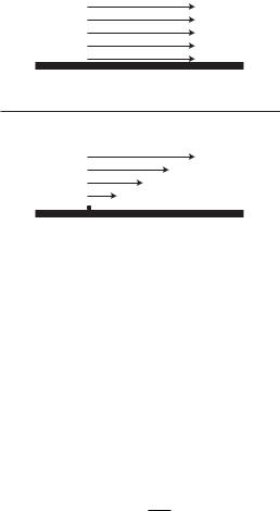
An important consequence of the viscous property of fluids is that the velocity di erence between adjacent layers of the fluid must be infinitely small so that the velocity gradient remains finite. In other words, change of velocity within the fluid must be smooth. A step change of velocity (Fig. 2.4.1) is not possible because it would produce a locally infinite velocity gradient, and the shear stress required to maintain it would be infinite (Eq. 2.4.1).

It follows from this property that at the interface between a moving fluid and a solid boundary, as at the inner surface of a tube, there can be no finite di erence between the fluid velocity tangential to the boundary and the

2.4 Fluid Viscosity: Resistance to Flow										43

Fig. 2.4.1. An important consequence of the viscous property of fluids is that the velocity di erence between adjacent layers of fluid must be infinitely small so that the velocity gradient remains finite. Thus, a step change of velocity (top) is not possible because it would produce a locally infinite velocity gradient and the shear stress required to maintain it would be infinite. Instead, the change of velocity must occur smoothly (bottom) so that the velocity gradient remains finite.

boundary itself. That is, the tangential velocity of fluid elements in contact with the boundary must be zero relative to the boundary, as required by the no-slip boundary condition (Fig. 2.4.2). This does not “prove” the noslip boundary condition but shows only that the viscous property of fluids is consistent with it. Indeed, the basis of the no-slip boundary condition has been and remains largely empirical [13, 34, 174, 71].

Eq. 2.4.1 applied to Poiseuille flow in a tube, with velocity u as given by Eq. 2.3.1, yields the following result for the shear stress τw at the tube wall

τw = μ	du	=	ka		=	aΔp		(2.4.2)
	dr		2			2l
		r=a

Since the pressure gradient k or pressure di erence Δp are negative in the flow direction, it follows that τw is also negative. That is, the shear stress (acting on the fluid) at the tube wall has the e ect of opposing the flow. The velocity gradient at the tube wall which is responsible for this shear stress is of course a consequence of the condition of “no-slip” there. It causes fluid in contact with the tube wall to come to rest while fluid along the tube axis charges at maximum velocity. A velocity gradient must therefore exist between the two regions and at the tube wall. Therefore, the condition of no-slip and the viscous property of the fluid together produce the shear stress at the tube wall.

44 2 Modelling Preliminaries

Fig. 2.4.2. The viscous property of fluids requires that at the interface between a moving fluid and a solid boundary, as at the inner surface of a tube, there be no finite di erence between the fluid velocity tangential to the boundary and the boundary itself (top). That is, the tangential velocity of fluid elements in contact with the boundary must be zero relative to the boundary itself (bottom), as required by the no-slip boundary condition.

The total resistance to flow R, which results from shear stress acting on the entire surface area of the tube, can be expressed in terms of the flow rate q as

	R =	Δp	(2.4.3)
		q

and substituting for the flow rate from Eq. 2.3.4, and using Eq. 2.3.2, this gives

R = −	8μl	(2.4.4)
	πa4

The minus sign indicates that the resistance, which represents the force exerted by the tube wall on the fluid, is opposite to flow direction. The sign is usually omitted because the term “resistance” in fact refers to a force opposing the flow, that is a force in the negative direction when flow represents the positive direction. This is equivalent to modifying the definition of R to

R = −	Δp	=	8μl	(2.4.5)
	q		πa4

It is seen that resistance to flow, which represents the amount of pressure di erence required to produce a given amount of flow, depends critically on tube radius, being proportional to the inverse of the radius to the fourth power. Thus, if the tube radius is reduced by a factor of 2, the resistance increases by a factor of 16, that is by 1, 600%. If the tube radius is increased by a factor of 2, the resistance decreases by a factor of 16, that is by approximately 94%.

2.5 Fluid Inertia: Inductance

45

Writing Eq. 2.4.5 as an equation for the flow rate q, we find the amount of flow that would be produced by a given pressure di erence Δp, namely

q = −	πa4Δp	(2.4.6)
	8μl

If in an experiment the amount of flow is found higher than that dictated by Eq. 2.4.6, this could be interpreted as a change in one of the other parameters on the right side of the equation. Indeed, experiments in the past have shown that there is an apparent drop in blood viscosity in very small blood vessels, usually referred to as the Fahraeus-Lindqvist e ect [63, 45, 221]. The e ect is termed “apparent” because it is not based on direct measurement of the viscosity μ but on a measurement of flow for a given pressure drop. Thus, an observed value of q higher than that prescribed by Eq. 2.4.6 was interpreted as a decrease in the viscosity μ because such a decrease would also produce a higher value of q. Another interpretation which has been considered is the possibility of partial slip at the tube wall which would have the e ect of requiring a smaller pressure drop for a given amount of flow, or conversely higher flow rate than is prescribed by Eq. 2.4.6, because of lower friction at the tube wall. However, it has been di cult to demonstrate that slip actually occurs in small blood vessels, and this interpretation is still a matter of debate [156, 211, 221]. Similar comments apply to the Fahraeus-Lindqvist e ect because of the di culties involved in actually measuring blood viscosity in small vessels. As a result of these di culties it has not been possible, so far, to incorporate the concepts of slip or of the Fahraeus-Lindqvist e ect into mainstream modelling schemes of the general dynamics of either the systemic or the coronary circulation.

2.5 Fluid Inertia: Inductance

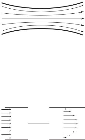
Acceleration in fluid flow may occur in one of two ways: in space or in time. Acceleration in space occurs when the space available to a stream of fluid is decreasing, so the fluid must increase its velocity to go through a reduced amount of space. Flow in a tube with a narrowing, as in a bottle neck, is an example (Fig. 2.5.1). Velocity at the narrowing must be higher than it is elsewhere, since the flow rate through the tube must be everywhere the same by conservation of mass, and since it is assumed here that the flow is incompressible, that is fluid density is not changing. Thus, the fluid is in a state of acceleration as it goes through the narrowing. The acceleration is in space, that is, in the sense that fluid elements are being accelerated as they progress along the tube.

Another, less obvious, example of acceleration in space occurs at the entrance to a tube. If fluid enters with uniform velocity (Fig. 2.5.2), elements of the fluid along the tube axis must accelerate to meet the maximum velocity

46 2 Modelling Preliminaries

Fig. 2.5.1. Flow in a tube with a narrowing causes fluid elements to accelerate as they approach the narrowing and decelerate as they leave, assuming that the fluid is incompressible. Flow velocity is highest at the neck of the narrowing as indicated by the closeness of the streamlines there. Both the acceleration and deceleration are occurring in space, in the sense that the change in velocity is occurring as fluid elements progress along the tube.

in Poiseuille flow, while fluid elements near the tube wall are slowed down by the viscous resistance to meet the condition of no-slip at the tube wall. Thus in the entrance region of the tube some fluid is in a state of acceleration and some is in a state of deceleration, in both cases the change is occurring in space, that is as the fluid progresses along the tube.

Fig. 2.5.2. Flow in the entrance region of a tube provides another example of acceleration and deceleration in space. If fluid enters with uniform veleocity, elements of the fluid along the tube axis must accelerate to meet the maximum velocity in Poiseuille flow, while fluid elements near the tube wall are slowed down by the viscous resistance and condition of no-slip at the tube wall.

One of the most important features of acceleration or deceleration in space is that it occurs in steady flow, that is, in a state of flow which does not change in time. In steady flow the velocity field does not change with time, meaning that the velocities at fixed positions within the flow field are constant and acceleration and deceleration occur as fluid elements move from one position to the next. It is in this sense that acceleration and deceleration in steady flow are seen as occurring in space.

Acceleration or deceleration in time, by contrast, is associated with unsteady flow, a state of flow in which the velocity distribution within the flow field changes with time. This situation occurs when the pressure driving the