The Physics of Coronory Blood Flow - M. Zamir

98 3 Basic Lumped Elements

p2

p = p2 - p1

R

C

p1 p1

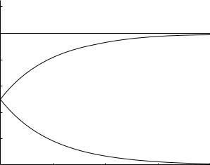
Fig. 3.6.1. Resistance R and capacitance C in parallel, under a pressure drop Δp. Resistance is represented here by a fully developed flow in a tube in which the only opposition to flow is the viscous resistance at the tube wall but with no inertial e ect since the flow is fully developed. Capacitance is represented by an expandable “balloon” in which the viscous resistance is absent but a capacitance e ect is present. The pressure drop across the resistance tube acts to overcome the viscous resistance at the tube wall, while across the balloon (p2 inside and p1 outside) it acts to keep it inflated and, depending on whether and how Δp is changing, it may drive flow into or out of the balloon, as discussed in Section 2.6.

as before and in subsequent analysis, we always assume that the balloon has not reached this limit and that flow is occuring within the elastic range of the balloon. This assumption is fairly consistent with physiological reality where the part of blood flow that goes into stretching blood vessels normally does so within their elastic limits. There have been suggestions that vessel walls may in fact be not purely elastic but viscoelastic [204, 52], but this issue is not important for the purpose of the present section.

Using the results established in Section 2.6, the two parallel flow rates are related to Δp by

1

Δp = qRR =

qC dt

(3.6.1)

C

or

qR =

Δp

(3.6.2)

R

qC = C

d(Δp)

(3.6.3)

dt

and total flow is given by

q = qR + qC

=

Δp

+ C

d(Δp)

(3.6.4)

R

dt

			3.6 R,C in Parallel	99
	Under a scenario of constant pressure drop Δp, we have
	qC = 0
	qR = q =	Δp		(3.6.5)
		R

Capacitive flow is zero because Δp is constant, and resistive flow is equal to total flow through the system.

Under the alternate scenario of constant total flow rate q into the system, the pressure drop Δp is no longer constant, as it must adjust in such a way as to maintain the prescribed constant flow rate q. This behaviour of Δp is

governed by the following di erential equation, from Eq. 3.6.4
C	d(Δp)	+	Δp		= q	(3.6.6)
	dt			R

which has the following solution, noting that q here is a constant

Δp(t) = qR + Ae−t/tC

(3.6.7)

where A is a constant and, as before, tC = RC. Using this result for the individual flows in Eqs.3.6.2,3, we obtain

qR(t) = q +			A	e−t/tC	(3.6.8)
			R
qC (t) = −	A				(3.6.9)
		e−t/tC
	R

To examine the interplay between capacitive and resistive flow rates we begin with the two being equal and follow their subsequent time course. In other words we set

qR(0) = qC (0)			(3.6.10)
which gives
A = −	Rq		(3.6.11)
	2

Using this value of A in Eqs.3.6.8,9, the flow rates can now be put in the following nondimentional forms

qR

1

qR(t) =

= 1 −

e−t/tC

(3.6.12)

q

2

C (t) =

qC

=

1

e−t/tC

(3.6.13)

q

q

2

=

q

= 1

(3.6.14)

q

q

100 3 Basic Lumped Elements

flow rate (nondimensionalized)

1.2
1			q
0.8			qR
0.6
0.4
0.2			qC
00		1	2	3	4
			t / tC

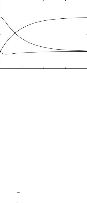
Fig. 3.6.2. Flow rates qR, qC in a resistive tube and a capacitive chamber (balloon), respectively, in parallel and under a condition of constant flow rate q through the system, normalized at a value of 1.0. At time t = 0 resistive and capacitive flows are set at normalized values of 0.5 each. Subsequently, capacitive flow diminishes from this value to an ultimate value of zero, while resistive flow increases gradually to ultimately encompass total flow into the system. Recalling that resistive flow is driven by the pressure drop while capacitive flow is driven by the derivative of the pressure drop, these changes in flow rates are accompanied by corresponding changes in the pressure drop and its derivative as described in the text.

recalling again that under the present scenario q is constant. The results are shown in Fig. 3.6.2, where we see that as time goes on, capacitive flow diminishes while resistive flow increases gradually to encompass total flow into the system. The reason for this can be seen from the behaviour of the pressure drop Δp as time goes on. From Eqs.3.6.7,11 we have

						1
Δp(t) = qR		1 −				2	e−t/tC	(3.6.15)
and by di erentiation
Δp (t) =		1		qR	e−t/tC			(3.6.16)
		2 tC

We recall from Section 2.6 that capacitive flow is driven not by the pressure drop Δp but by the rate of change of the pressure drop, namely Δp (t). Accordingly, from Eq. 3.6.16 we see that Δp (t) has its maximum value at time t = 0 and diminishes continuously thereafter to an ultimate value of zero. Consequently, capacitive flow has its maximum value at time t = 0 and then

3.7 RLC System in Parallel Under Constant Pressure

101

diminishes gradually to an ultimate value of zero. Since total flow into the system is constant under the present scenario, resistive flow begins with its lowest value at time t = 0 and then increases gradually to encompass total flow into the system, as illustrated in Fig. 3.6.2. Interestingly, the corresponding change in the pressure drop is such that it actually increases from its initial value to the value required to drive the ultimate resistive flow, but the derivative of the pressure drop (which drives the capacitive flow) decreases continuously from its initial value to an ultimate value of zero.

3.7 RLC System in Parallel Under Constant Pressure

Finally, we conclude this chapter, which started out by considering the three elements of resistance R, inductance L, and capacitance C, in series, by considering now these three elements in parallel under a driving pressure drop Δp as shown in Fig. 3.7.1. As before, the pressure drop will act to overcome the viscous e ect in the resistive tube, the inertial e ect in the inductive tube, and the capacitance e ect in the balloon (capacitor).

p2

p = p2	- p1	R	L	C

p1 p1 p1

Fig. 3.7.1. Resistance R, inductance L, and capacitance C, in parallel under a pressure drop Δp, other details as in Fig. 3.5.1 and Fig. 3.6.1.

If, as in Sections 3.5,6, resistive, inductive, and capacitive flow rates are denoted by qR, qL, qC , respectively, then, as before, these are related to the pressure drop by

Δp = qRR					(3.7.1)
= L		dqL			(3.7.2)
			dt
1
=				qC dt	(3.7.3)
	C

102 3 Basic Lumped Elements
or
qR =	Δp
	R
qL = L				Δpdt
	1

qC = C d(Δp)

dt

Total flow rate into the parallel system is given by

q = qR + qL + qC
= R		+ L		Δpdt + C	dt
	Δp	1			d(Δp)

(3.7.4)

(3.7.5)

(3.7.6)

(3.7.7)

(3.7.8)

and, after di erentiation, we have the following di erential equation governing the dynamics of the system

dq		1 d(Δp)				Δp		d2(Δp)
	=				+		+ C		(3.7.9)
dt								dt2
	R dt					L

For the purpose of obtaining solutions of this equation, it is convenient to put it in the following form, using the inertial and capacitive time constants introduced in earlier sections

	d2(Δp)		d(Δp)		1		dq
tC		+			+		Δp = R		(3.7.10)
	dt2			dt		tL		dt
where, as before
				tL = L/R					(3.7.11)
				tC = CR					(3.7.12)

Under the scenario of constant pressure drop (Δp = constant), Eq. 3.7.10 reduces to

	dq	=		1		Δp	(3.7.13)
	dt				L
with the solution
q(t) =			Δp			t + A	(3.7.14)
				L

where A is a constant. Also, from Eqs.3.7.4-6, with Δp constant, we have

	qR(t) =	Δp		(3.7.15)
		R
	qL(t) =	Δp	t + B	(3.7.16)
		L
	qC (t) = 0			(3.7.17)

3.8 RLC System in Parallel Under Constant Flow

103

where B is a constant. If at time t = 0 it is assumed that fluid in the inductance tube is at rest, that is qL(0) = 0, then B = 0 and

qL(t) =	Δp	t	(3.7.18)
	L

Total flow rate through the parallel system is thus given by

q(t) = qR(t) + qL(t) + qC (t)

=	Δp	+	Δp	t	(3.7.19)
	R
			L

and comparing this with Eq. 3.7.14 we see that A = Δp/R and the two equations become identical, as they should. Thus, under the scenario of constant pressure drop, the individual and total flow rates, in nondimensional form, are given by

				(t) =	qR(t)	= 1
	q	R
				Δp/R
				(t) =	qL(t)	=	t
	q	L
				Δp/R			tL
		C (t) = 0
q
				(t) =	q(t)	= 1 +			t
			q
									tL
				Δp/R

(3.7.20)

(3.7.21)

(3.7.22)

(3.7.23)

These results are identical with those obtained in Section 3.5, Eq. 3.5.12, and shown in Fig. 3.5.2. Thus, under a scenario of constant pressure drop, the LRC system in parallel is the same as the LR system in parallel. The reason for this, of course, is that capacitive flow is driven not by Δp but by changes in Δp.

3.8 RLC System in Parallel Under Constant Flow

With a constant flow rate, that is a constant total flow rate into the parallel system, setting q constant in Eq. 3.7.10, the equation reduces to

	d2(Δp)		d(Δp)		1
tC		+			+		Δp = 0	(3.8.1)
	dt2			dt		tL

This is a standard second order linear homogeneous di erential equation with constant coe cients [116]. Its solution depends on the roots of the associated (so-called “indicial”) equation

tC α2 + α +	1	= 0	(3.8.2)
	tL

104	3 Basic Lumped Elements
The roots are in general given by
			2tC
	α =	−1 ±	1 − (4tC /tL)	(3.8.3)

but the solution of the governing equation (Eq. 3.8.1) and hence the dynamics of the system depend critically on whether these roots are real or complex, which in turn depends on the relative values of the inertial and capacitive time constants tL, tC .

If 4tC < tL, then Eq. 3.8.2 has two distinct real roots, given by

	1		−				2tC
α		=		1 +			1	− (4tC /tL)
	2		−		−
							2tC
α		=		1			1	− (4tC /tL)

and the solution of the governing equation (Eq. 3.8.1) is given by

Δp(t) = Aeα1t + Beα2t

(3.8.4)

(3.8.5)

(3.8.6)

where A, B are arbitrary constants. Using this result for Δp in Eqs. 3.7.4–6, we find

qR(t) =

Δp(t)

R

=

A

eα1t +

B

eα2t

(3.8.7)

R

R

qL(t) = L Δp(t)dt

1

=

A

eα1t +

B

eα2t + K

(3.8.8)

Lα1

Lα2

qC (t) = C

d(Δp(t))

dt

= ACα1eα1t + BCα2eα2t

(3.8.9)

where K is a constant of integration. Using the condition of constant total flow rate under the present scenario, namely

qR(t) + qL(t) + qC (t) = q (constant)

(3.8.10)

we find, after some algebra,

K = q

(3.8.11)

The flow rates in Eqs.3.8.7-9 can now be put in the following nondimensional form:

3.8 RLC System in Parallel Under Constant Flow 105

(t) =

qR(t)

=

(3.8.12)

R

Aeα1t + Beα2t

q

q

qL(t)

L

(t) =

=

A

eα1t +

B

eα2t + 1

(3.8.13)

q

q

tLα1

tLα2

(t) =

qC (t)

=

eα1t +

eα2t

(3.8.14)

At

α

Bt

α

q

C

C

C

q

1

2

where

=

A

(3.8.15)

A

Rq

=

B

(3.8.16)

B

Rq

The pressure drop can also be put in nondimensional form by writing

(t) =

Δp

=

(3.8.17)

Δp

Aeα1t + Beα2t

Rq

from which we note that, in their nondimensional form, the pressure drop Δp and the resistive flow qR are the same function of time (Eqs. 3.8.12, 17).

The constants A, B can be determined in terms of prescribed values for

the initial flow rates by setting t = 0 in Eqs. 3.8.12–14, to get

R(0)

=

+

(3.8.18)

A

B

q

A

B

q

L(0)

=

+

+ 1

(3.8.19)

tLα1

tLα2

C (0)

=

(3.8.20)

AtC α1 + BtC α2

q

Since there are three initial flow rates and only two unknown constants, only two of the flow rates can be prescribed. There are a number of di erent combinations in which this can be done. From a practical standpoint we may assume that at time t = 0 the entire inflow q is going through the resistive tube while the sum of the inductive and capacitive flow rates is zero, that is

		q		R(0)	= 1	(3.8.21)
	L(0) +		C (0)		= 0	(3.8.22)
q		q

From a strictly mathematical standpoint, this is equivalent to setting

q		R(0)		= 1	(3.8.23)
			L(0)	= x	(3.8.24)
q
	C (0)			= −x	(3.8.25)
q

106 3 Basic Lumped Elements

where x is as yet unknown. The second and third of these conditions can now be used to find A, B in terms of x, and the first equation can then be used to find the value or values of x that would satisfy that equation. When this is done, we find in fact that all values of x satisfy this condition. From a practical standpoint, the choice x = 0 is appropriate since it can be achieved by having a pre-existing constant flow rate q through the resistive tube at time t < 0 with the entrances to the inductive and capacitive tubes closed, then at time t = 0 these entrances are opened. And if the choice x = 0 is to be made, then we may find A, B by simply setting the initial conditions

			q		L(0)		= 0	(3.8.26)
				C (0)			= 0	(3.8.27)
		q
which give, after some algebra
							α2
	A =							(3.8.28)
						α2 − α1
			=			−α1		(3.8.29)
	B
						α2 − α1

We note that these values satisfy the condition A + B = 1 in Eq. 3.8.18, as well as the condition q(0) = qR(0) + qL(0) + qC (0) = 1 required under the present scenario of constant flow rate into the parallel system. With these values of A, B, the solution is now complete, and the nondimensional flow rates in Eqs.3.8.12-14 can be plotted as functions of time. Values of the time constants tL, tC are required in order to complete the process. Results using tL = 1.0, tC = 0.1, are shown in Fig. 3.8.1. It is seen that at time t = 0 the inductive and capacitive flow rates have the prescribed nondimensional values qL = qC = 0, while the resistive flow rate, as a consequence, has the value 1.0. Thus, initially all flow is going through the resistive tube, but fairly soon thereafter this flow diminishes while the inductive flow grows to encompass total flow into the system. Capacitive flow is very small throughout this process, and it too becomes zero as time goes on.

If 4tC > tL, then Eq. 3.8.2 has two complex (conjugate) roots, given by

	α1			= a + ib			(3.8.30)
	α2			= a − ib			(3.8.31)
where
a = −1/2tC							(3.8.32)
b =
					2tC	−	(3.8.33)
				(4tC /tL)			1
i =	√						(3.8.34)
			−1

flow rate (normalized)

		3.8 RLC System in Parallel Under Constant Flow					107
1.5
1
		qL
0.5
		qR,	p
0		qC
−0.50
		1	2	3	4
			t / tL

Fig. 3.8.1. Flow rates qR, qL, qC in a resistive tube, an inductive tube, and a capacitive chamber (capacitor), in parallel under a condition of constant flow rate q into the system, normalized at a value of 1.0. At time t = 0 inductive and capacitive flows are set at zero, and by consequence resistive flow has an initial value of 1.0, that is, the resistive tube intially carries the entire flow rate into the system. Subsequently, however, the situation reverses as inductive flow grows rapidly to encompass the entire flow into the system. Since under the present scenario total flow into the system is fixed at a normalized value of 1.0, capacitive and resistive flow rates diminish to zero as a consequence. The way in which the flow rates approach their ultimate values depends on the values of the inertial and capacitive time constants tL, tC . Results in this figure are based on tL = 1.0, tC = 0.1.

and the solution of the governing equation (Eq. 3.8.1) is given by

Δp(t) = eat{A cos(bt) + B sin(bt)}

(3.8.35)

where A, B are arbitrary constants. Using this result for Δp in Eqs. 3.8.7–9, we find, after a considerable amount of algebra,

qR(t) =	Δp
	R
	eat
=		{A cos(bt) + B sin(bt)}		(3.8.36)
	R

1

qL(t) = L Δp(t)dt

=eat {A(− cos(bt) + 2btC sin(bt)) 2R