198 ION–SENSITIVE FIELD-EFFECT TRANSISTORS
the mouth of patients with xerostomia. IEEE Trans Biomed Eng 1991;38:353–356.
59.Hiraishi N, et al. Evaluation of active and arrested carious dentin using a pH-imaging microscope and an X-ray analytical microscope. Oper Dent 2003;28:598–604.
60.De Aza PN, Luklinska ZB, Anseau M. Bioactivity of diopside ceramic in human parotid saliva. J Biomed Mater Res Part B 2005;73B:54–60.
61.Sant W, et al. Development of a creatinine-sensitive sensor for medical analysis. Sens Actuator B-Chem 2004;103:260–264.
62.Mackay RS. Radio telemetering from within the body. Science 1961;134:1196–1202.
63.Iddan G, Meron G, Glukhovsky A, Swain P. Wireless capsule endoscopy. Nature (London) 2000;405:417–417.
64.Pandolfino JE, et al. Ambulatory esophageal pH monitoring using a wireless system. Am J Gastroenterol 2003;98:740–749.
65.Johannessen EA, et al. Implementation of multichannel sensors for remote biomedical measurements in a microsystems format. IEEE Trans Biomed Eng 2004;51:525–535.
See also IMMUNOLOGICALLY SENSITIVE FIELD-EFFECT TRANSISTORS;
INTEGRATED CIRCUIT TEMPERATURE SENSOR.
ISFET. See ION-SENSITIVE FIELD-EFFECT TRANSISTORS.

J
JOINTS, BIOMECHANICS OF
GEORGE PAPAIOANNOU
University of Wisconsin
Milwaukee, Wisconsin
YENER N. YENI
Henry Ford Hospital
Detroit, Michigan
INTRODUCTION
The human skeleton is a system of bones joined together to form segments or links. These links are movable and provide for the attachment of muscles, ligaments, tendons, and so on. to produce movement. The junction of two or more bones is called an articulation. There are a great variety of joints even within the human body and a multitude of types among living organisms that use exoand endoskeletons to propel. Articulation can be classified according to function, position, structure and degrees of freedom for movement they allow, and so on. Joint biomechanics is a division of biomechanics that studies the effect of forces on the joints of living organisms.
Articular Anatomy, Joint Types, and Their Function
Anatomic and structural classification of joints typically results in three major categories, according to the predominant tissue or design supporting the articular elements together, that is, joints are called fibrous, cartilaginous, or synovial.
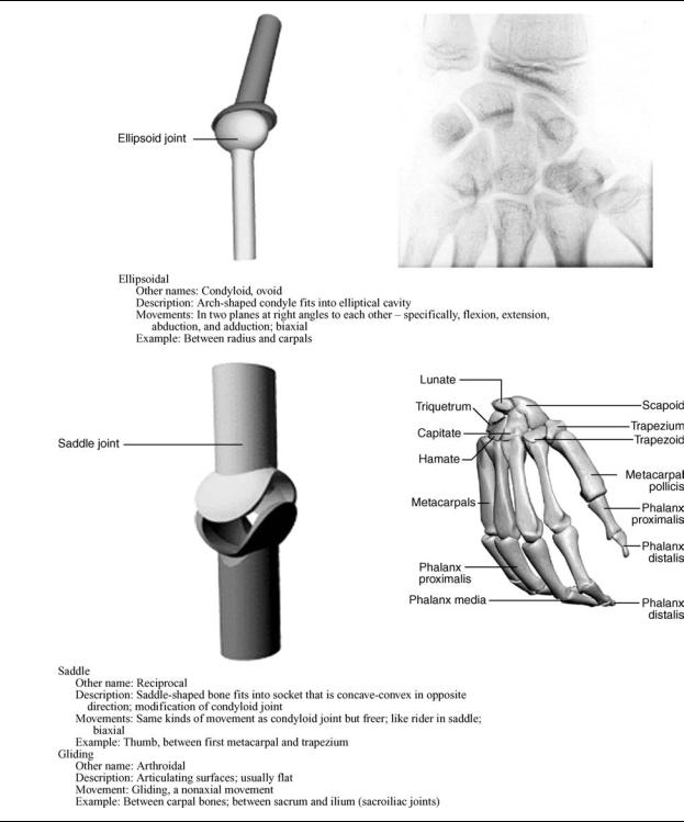
Synovial joints are cavitated. In general, two rigid skeletal segments are brought together by a capsule of connective tissue and several other specialized tissues, that form a cavity. The joints of the lower and upper limbs are mainly synovial since these are the most mobile joints. Mobility varies considerably and a number of subcategories are defined based on the specific shape or architecture and topology of the surfaces involved (e.g., planar, saddle, ball and socket) and on the types of movement permitted (e.g., flexion and extension, medial and lateral rotation) (Table 1). The basic structural characteristics that define a synovial joint can be summarized in four features: a fibrous capsule that forms the joint cavity, a specialized articular cartilage covering the articular surfaces, a synovial membrane lining the inner surface of the capsule that also secretes a special lubricating fluid, the synovial fluid. Additional supportive structures in synovial joints include disks, menisci, labra, fat pads, tendons, and ligaments.
Cartilaginous joints are also solid and are more commonly known as synchondroses and symphyses, a classification based on the structural type of cartilage that intervenes between the articulating parts (Table 2). This cartilage is hyaline and fibrocartilage for synchondroses and symphyses, respectively. Synchondroses allow very
little movement as in the case of the rib cage that contributes to the ability of this area to expand with respiration. Most symphyses are permanent; those of sacrum and coccyx can, however, degenerate with subsequent fusion between adjacent vertebral bodies as part of the normal development of these bones.
Fibrous joints are solid. The binding mechanism that dominates the connectivity of the articulating elements is principally fibrous connecting tissue, although other tissue types also may be present. Length, specific arrangement, and fiber density vary considerably according to the location of the joint and its functional requirements. Fibrous joints are classified in three groups: sutures, gomphoses, and syndesmoses (Table 3);
In addition to the obligatory components that all the synovial joints possess, several joints contain intraarticular structures. Discs and menisci are examples of such structures. They differ from one another mainly in that a disc is a circular structure that may completely subdivide a joint cavity so that it is, in reality, two joints in series, whereas a meniscus is usually a crescent-shaped structure that only partially subdivides the joint. Complete discs are found in the sternoclavicular and in the radiocarpal joint. A variety of functions have been proposed for intraarticular discs and menisci. They are normally met at locations where bone congruity is poor, and one of their main functions is to improve congruity and, therefore stability between articular surfaces. Shock absorption facilitation and combination of movements are among their likely roles. They may limit a movement or distribute the weight over a larger surface or facilitate synovial fluid circulation throughout the joint.
The labrum is another intraarticular structure. In humans, this structure is only found in the glenohumeral and hip joints. They are circumferential structures attached to the rim of the glenoid and acetabular sockets. Labra are distinct from articular cartilage because they consist of fibrocartilage and are triangular in their middle section. Their bases are attached to the articular margins and their free apical surfaces lined by synovial membrane. Like discs, their main function is to improve fit and protect the articular margins during extremes of movement.
Fat pads are localized accumulations of fat that are found around several synovial joints, although only those in the hip (acetabular pad) and the knee joint (infrapatellar pad) are named. Suggested functions for fat pads include protection of other intraarticular structures (e.g., the round ligament of the head of the femur) and serving as cushions or space-fillers thus facilitating more efficient movement throughout the entire available range.
Bursae are enclosed, self-contained, flattened sacs typically with a synovial lining. They facilitate movement of musculoskeletal tissues over one another and thus are located between pairs of structures (e.g., between ligament and tendon, two ligaments, two tendons or skin, and bone). Deep bursae, such as the illiopsoas bursa or the deep
199

Table 1. Diarthroses: Synovial Joints
200
JOINTS, BIOMECHANICS OF |
201 |
Table 1. (Continued )
retrocalcaneal bursa, develop along with joints and by a similar series of events during the embryonic period.
Tendons are located at the ends of many muscles and are the means by which these muscles are attached to bone or other skeletal elements. The primary structural component of tendons is type I collagen. Tendons almost exclusively operate under tensile forces.
Ligaments are dense bands of connective tissue that connect skeletal elements to each other, either creating (as in the case of syndesmoses) or supporting joints. According to their location they are classified as intracapsular, capsular, or extracapsular. Structurally, they resemble the tendons in that they consist predominantly of type I collagen.

202 JOINTS, BIOMECHANICS OF
Table 2. Amphiarthroses: Cartilaginous Joints
Articular Cartilage
Articular cartilage, the resilient load-bearing tissue that forms the articulating surfaces of synovial joints functions through load distribution mechanism by increasing the area of contact (thereby reducing the stress) and provides these surfaces with the low friction, lubrication, and wear characteristics required for repetitive gliding motion.
Biomechanically, cartilage is another intraarticular absorption mechanism that dampens mechanical shocks and spreads the applied load onto subchondral bone (Fig. 2). Articular cartilage should be viewed as a multiphasic material. It consists primarily of a large extracellular matrix (ECM) with a sparse population of highly specialized cells (chondrocytes) distributed throughout the tissue. The
primary components of the ECM are water, proteoglycans, and collagens, with other proteins and glycoproteins present in lower amounts (1). The solid phase is comprised by this porous-permeable collagen-PG matrix filed with freely movable interstitial fluid (fluid phase) (2). A third phase is the ion phase, necessary to describe the electromechanical behaviors of the system. The structure and composition of the articular cartilage vary throughout its depth (Fig. 2), from the articular surface to the subchondral bone. These differences include cell shape and volume, collagen fibril diameter and orientation, proteoglycan concentration, and water content. These all combine to provide the tissue with its unique and complex structure and mechanical properties. A fine mechanism of interstitial fluid pressurization

JOINTS, BIOMECHANICS OF |
203 |
Table 3. Synarthroses: Fibrous Joints
Figure 1. Basic structure and components of a synovial joint (also called diarthroses).
Figure 2. Zones of articular cartilage.
204 JOINTS, BIOMECHANICS OF
results from the flow of interstitial fluid through the porouspermeable solid matrix that in turn defines the rate dependent load-bearing response of the material. It is noteworthy that articular cartilage provides its essential biomechanical functions for eight decades or more in most of the human synovial joints and no synthetic material performs this well as a joint surface.
The frictional characteristics between two surfaces sliding over each other are significantly influenced by the topography of the given surfaces. Anatomical shape changes affect the way in which loads are transmitted across joints, altering the lubrication mode in that joint and, thus, the physiologic state of cartilage. Articular surfaces are relatively rough, compared to machined bearing surfaces, at the microscopic level. The natural surfaces are surprisingly much rougher than joint replacement prostheses. The mean of the surface roughness for articular cartilage ranges from 1 to 6 mm, while the metal femoral head of a typical artificial hip has a value of 0.025 mm, indicating that the femoral head is apparently much smoother. Topographic features on the joint surfaces are characterized normally by primary anatomic contours, secondary roughness (<0.5 mm in diameter and <50 mm deep), tertiary hollows on the order of 20–45 mm deep; and, finally, quaternary ridges 1–4 mm in diameter and 0.1–0.3 mm deep. Scanning electron micrographs (SEMs)of arthritic cartilage usually depict a large degree of surface irregularity and anomalous microtopography. These surface irregularities have profound effects on the lubrication mechanism. They accelerate the effects of friction and the rate of degradation of the articular cartilage. The types of joint surface interactions vary greatly between different joints in the body, different animals, between different size animals of the same species, different genders, and different ages. For example, the human hip joint is a deep congruent ball and socket joint (where the cartilage thickens peripherally at the acetabulum); this differs greatly from the bcondylar nature of the distal femur in the knee joint, and the saddle shape of the carpometacarpal joint in the thumb. The degree of shape matching between the various bones and articulating cartilage surfaces composing a joint is a major factor affecting the distribution of stresses in the cartilage and subchondral bone.
Effects of Motion and External Loading on Joints
The articular joint is viewed as an organ with complicated mechanisms of memory and adaptation that accommodates changes in its function. Joint loading results in motion and the couple load–motion is required to maintain normal adult articular cartilage composition, structure, and mechanical properties. The type, intensity, and frequency of loading necessary to maintain normal articular cartilage vary over a broad range. The intensity or frequency of loading should not exceed or fall below these necessary levels, since this will disturb the balance between the processes of synthesis and degradation. Changes in the composition and microstructure of cartilage will result. Reduced joint loading, as has been observed in cases of immobilization by casting or external fixation, leads to atrophy or degeneration of the cartilage. The
changes affect both the contact and noncontact areas. Changes in the noncontact areas resulting from rigid immobilization include fibrillation, decreased proteoglycan content and synthesis, and altered proteoglycan conformation, such as a decrease in the size of aggregates and amount of aggregate. Normal nutritive transport to cartilage from the synovial fluid by means of diffusion and convection has been diminished, resulting in these changes. Increased joint loading, either through excessive use, increased magnitudes of loading, or impact, also may affect articular cartilage. Catabolic effects can be induced by a single-impact or repetitive trauma, and may serve as the initiating factor for progressive degenerative changes. Osteoarthritis, a joint disease of epidemic proportions in the western world, is characterized by erosive cartilage lesions, cartilage loss and destruction, subchondral bone sclerosis and cysts, and large osteophyte formation at the margins of the joint (3).
Moderate running exercise may increase the articular cartilage proteoglycan content and compressive stiffness, decrease the rate of fluid flux during loading, and increase the articular cartilage thickness in skeletally immature animals. However, no significant changes in articular cartilage mechanical properties were observed in dogs in response to lifelong increased activity that did not include high impact or torsional loading of their joints. Disruption of the intraarticular structures (e.g., menisci or ligaments) will alter the forces acting on the articular surface in both magnitude and areas of loading. The resulting joint instability is associated with profound and progressive changes in the biochemical composition and mechanical properties of articular cartilage. In experimental animal models, responses to transection of the anterior cruciate ligament or meniscectomy have included fibrillation of the cartilage surface, increased hydration, changes in the proteoglycan content, reduced number and size of proteoglycan aggregates, joint capsule thickening, and osteophyte formation. It seems likely that some of these changes result from the activities of the chondrocytes, because their rates of synthesis of matrix components, breakdown of matrix components, and secretion of proteolytic enzymes are all increased. In vitro studies have shown that loading of the cartilage matrix can cause all of these mechanical, electric, and physicochemical events, but thus far it has not been clearly demonstrated which signals are most important in stimulating the anabolic and catabolic activity of the chondrocytes. A holistic physicochemical and biomechanical model of cartilage function in health and disease remains a challenge in the scientific community.
KINEMATICS OF JOINTS
General Comments
Mechanical analysis can refer to kinetics (forces) and/or kinematics (movement), with kinetics being the cause and kinematics the result. Mechanical analysis can develop models proceeding from forces to movements or vice versa. The analysis that starts from the cause (force) is called direct or forward dynamics, and produces a defined set of forces that caused the unique movement. This approach has one solution, and hence is deterministic. Starting from
the movement the analysis is called inverse dynamics. In this case, an infinite number of combinations of individual forces acting on the system can be the causes of the same unique movement, which makes the inverse dynamics approach not deterministic. The simplest and most essential system of mechanical formulations for explaining and describing motion is the Newton’s second law. More advanced techniques include the Lagrange, d’Alembert, and Hamilton’s methods. In general all of these methods start by describing equations of motion for a rigid body for translation, rotation, or combinations of them for both two (2D) and three-dimensional (3D) space. If the model assumes that the articulated segments that create the articulation are modeled as rigid bodies the remaining task is to calculate the relative motion between the two segments by applying graphics or joint kinematic analysis.
Kinematics is the study of the movements of rigid structures, independent of the forces that might be involved. Two types of movement, translation (linear displacement) and rotation (angular displacement), occur within three orthogonal planes; that is, movement has six degrees of freedom. Humans belong to the vertebrate portion of the phylum chordata, and as such possess a bony endoskeleton that includes a segmented spine and paired extremities. Each extremity is composed of articulated skeletal segments linked together by connective tissue elements and surrounded by skeletal muscle. Motion between skeletal segments occurs at joints. Most joint motion is minimally translational and primarily rotational. The deviation from absolute rotatory motion may be noted by the changes in the path of a joint’s ‘‘instantaneous center of rotation’’. These paths have been measured for most of the joints in the body and vary only slightly from true arcs of rotation. For human motion to be effective, not only must a comparatively rigid segment rotate its position relative to an adjacent segment, but many adjacent limb movements must interact as well. Whether the hand is trying to write or the foot must be lifted high enough to clear an obstacle on the ground, the activity is achieved via coordinated movements of multiple limb segments. To provide for the greatest possible function of an extremity, the proximal joint must have the widest range of motion to position the limb in space. This joint must allow for rotatory motions of large degrees in all three planes about all three axes. A means is also provided to translate the limb, so that an extremity can function at all locations within its global range. Rotational motion of the elbow and knee joints allows such overall changes as adjacent limb segments move. Finally, to finetune the use of this mechanism with respect to the extremities, for their functional purposes, the hand and foot are required to have a vast amount of movement about all three axes, although the rigid segments are relatively small. Such movement requires the presence of relatively universal joints at the terminal aspect of each extremity.
Characterization of the General Mechanical Joint System:
Terminology and Definitions
The displacement of a point is simply the difference between its position after a motion and its position before that motion. It can be represented by a 3D vector drawn
JOINTS, BIOMECHANICS OF |
205 |
from the initial position of the point to its final position. The components of the displacement vector will be the changes in the coordinates of the point’s position from measurement in the reference coordinate system. It is apparent that not only the positions, but also displacements measured are relative to some reference. Rigid body (RB) displacements are more complicated than point displacements since for a rigid body a displacement is a change in its position relative to some reference, but more than three parameters are needed to describe it. Two simple types of RB displacement can be described: translation and rotation. An important property of pure translation of a RB is that the displacement vectors of all points in the body are identical and are nonzero. In pure rotation of a RB, although points in the body experience nonzero displacements, one point in that body experiences zero displacement. In addition to that rule, Euler’s theorem shows that in pure rotation all points along a particular line through that undisplaced point also experience zero displacement. This line is also known as the axis of rotational displacement. Chasles theorem further states that any displacement of a RB can be accomplished by a translation along a line parallel to the axis of rotation that is defined by Euler’s theorem plus a rotation about that same parallel axis. Simply that suggests that any displacement in 3D isequivalent to the motion of a nut,representing the body, on an appropriate stationary screw that was centered on the line described above. Indeed, it can be shown that any displacement in 3D is equivalent to a translation plus a rotation.
Degrees of Freedom
The biological organisms capable of propelling themselves through different media consist of more than one rigid body. A system consisting of a 3D reference frame and an isolated rigid body in space has six degrees of freedom (DOF). To describe the position of each body relative to the ground reference frame it would be necessary to use six parameters, so for two unconnected rigid bodies 12 parameters would be necessary. The system consisting of these two unconnected bodies and the fixed -ground reference would have 12 DOF. The human–animal body consists of a combination of suitably connected bodies. The connections, joints between the bodies, serve to constrain the motions of the bodies so that they are not free to move with what would otherwise be six DOF for each body. Therefore, we can define the number of DOF that the joint removes as the number of degrees of constraint that it provides. It can be shown that every time a joint is added to a system, the number of degrees of freedom in that system is reduced by the number of degrees of constraint provided by that joint. This suggests the following generic formula for the calculation of the degrees of freedom of a system:
F ¼ 6ðL 1Þ 5J1 4J2 3J3 2J4 J5
where F ¼ is the number of degrees of freedom in the system of connected joints; L ¼ is the number of joints in the system, including the ground joint (which has no degrees of freedom), and Jn ¼ the number of joints having n degrees of freedom each.
Table 4 contains a description of the major joints in the human body along with the segments-bones that they
206 |
JOINTS, BIOMECHANICS OF |
|
|
|
|
|
Table 4. Characteristics of Major Human Joints |
|
|
|
|||
|
|
|
|
|
|
|
Joint |
|
Bones |
Type |
DOF |
Type of motion |
Range of Motion (deg) |
|
|
|
|
|
|
|
Shoulder |
|
Humerus-Scapula |
Diarthrosis (spheroidal) |
3 |
Flexion |
150 |
|
|
|
|
|
Extension |
50–60 |
|
|
|
|
|
Abduction |
90–120 |
|
|
|
|
|
Abduction |
Complete |
|
|
|
|
|
Rotation |
|
Elbow |
|
Humerus-ulna |
Diarthrosis (ginglymus) |
2 |
Flexion |
145–160 |
|
|
|
|
|
Extension |
0–5 |
|
|
|
|
|
Rotation (radius) |
|
Radioulnar |
Superior radius-ulna |
Diarthrosis (trochoid) |
1 |
Pronation |
70–75 |
|
|
|
|
|
|
Supination |
85–90 |
Wrist |
|
Radius-carpal |
Diarthrosis (condyloid) |
2 |
Flexion |
90–95 |
|
|
|
|
|
Extension |
60–70 |
|
|
|
|
|
Radial deviation |
20–25 |
|
|
|
|
|
Ulnar deviation |
55–65 |
|
|
|
|
|
Circumduction |
Complete |
Metacarpal-phalangeal |
Metacarpal-phalanges |
Diarthrosis (condyloid) |
2 |
Flexion |
80–90 |
|
|
|
|
|
|
Extension |
20–30 |
|
|
|
|
|
Radial deviation |
20–25 |
|
|
|
|
|
Ulnar deviation |
15–20 |
Finger |
|
Interphalanges |
Diarthrosis (ginglymus) |
1 |
Flexion |
80–90 |
|
|
|
|
|
Extension |
0–10 |
Thumb |
|
First metacarpal-carpal |
Diarthrosis (reciprocal) |
2 |
Flexion |
80–90 |
|
|
|
|
|
Extension |
20–25 |
|
|
|
|
|
Abduction |
40–45 |
|
|
|
|
|
Abduction |
0–10 |
|
|
|
|
|
Circumduction |
Complete |
Hip |
|
Femur-acetabulum |
Diarthrosis (spheroidal) |
3 |
Flexion |
90–120 |
|
|
|
|
|
Extension |
10–20 |
|
|
|
|
|
Abduction |
30–45 |
|
|
|
|
|
Abduction |
30 |
|
|
|
|
|
Medial rotation |
30–40 |
|
|
|
|
|
Lateral rotation |
60 |
|
|
|
|
|
Circumduction |
Complete |
Knee |
|
Tibia-femur |
Diarthrosis (ginglymus) |
2 |
Flexion |
120–140 |
|
|
|
|
|
Extension |
0 |
|
|
|
|
|
Medial rotation |
30 |
|
|
|
|
|
Lateral rotation |
40 |
Ankle |
|
Tibia-fibula-talus |
Diarthrosis (ginglymus) |
1 |
Flexion |
20–30 |
|
|
|
|
|
Extension |
40–45 |
Intertarsal |
Tarsals |
Diarthrosis (arthroidal) |
2 |
Gliding |
Limited motion |
|
Metatarsal-phalangeal |
Metatarsals-phalanges |
Diarthrosis (condyloid) |
2 |
Flexion |
25–30 |
|
|
|
|
|
|
Extension |
80–90 |
|
|
|
|
|
Abduction |
15–20 |
|
|
|
|
|
Abduction |
Limited |
Interphalangeal |
Phalanges |
Diarthrosis (arthroidal) |
1 |
Flexion |
90 |
|
|
|
|
|
|
Extension |
0 |
Tibio-fibular |
Distal tibia-fibula |
Synarthrosis (syndesmosis) |
0 |
Slight movement |
Give |
|
Skull |
|
Cranial |
Synarthrosis (suture) |
0 |
No movement |
|
Sterno-costal |
Ribs-sternum |
Amphiarthrosis (synchondrosis) |
0 |
Slight movement |
|
|
Sacroiliac |
|
Sacrum-ilium |
Amphiarthrosis (synchondrosis) |
0 |
No movement |
Elastic |
Intervertebral |
Cervical vertebrae |
Diarthrosis (arthroidal) |
3 |
Flexion |
40 |
|
|
|
|
|
|
Extension |
75 |
|
|
|
|
|
Lateral flexion |
35–45 |
|
|
|
|
|
Axial rotation |
45–50 |
|
|
Thoracic vertebrae |
Diarthrosis (arthroidal) |
3 |
Flexion |
105 |
|
|
|
|
|
Extension |
60 |
|
|
|
|
|
Lateral flexion |
20 |
|
|
|
|
|
Axial rotation |
35 |
|
|
Lumbar vertebrae |
Diarthrosis (arthroidal) |
3 |
Flexion |
60 |
|
|
|
|
|
Extension |
35 |
|
|
|
|
|
Lateral flexion |
20 |
|
|
|
|
|
Axial rotation |
5 |
|
|
Atlas axis |
Diarthrosis (trochoid) |
1 |
Pivoting motion |
|
|
|
|
|
|
|
|

articulate, their respective type DOF and type/range of motion they provide.
Planar Motion
Some human joints move predominantly in one plane (e.g., the knee joint) in which case the motion can be approximated and analyzed by graphical methods. Here the rotation is characterized by the motion of all points on concentric cycles with an identical angle of rotation around the undisplaced center of rotation (CR). The CR may be located inside and outside of the boundaries of the rotating body. The most common graphical method for the calculation is the so-called bisection technique. If the initial and final states of the body are known, the position of the center or rotation and the angle of rotation may be reconstructed (Fig. 3).
Instantaneous Center of Rotation
When a 2D body is rotating without translation, for example, a rotating stationary bicycle gear, any marked point P on the body may be observed to move in a circle about a fixed point called the axis of rotation or center of rotation. When a rigid body is both rotating and translating, for example, the motion of the femur during gait, its motion at any instant of time, can be described as rotation around a moving center of rotation. The location of this point at any instant, termed the instantaneous center of rotation (ICR), is determined by finding the point which, at that instant, is not translating. Then by definition, at that instant, all points on the rigid body are rotating about the ICR. For practical purposes, the ICR is determined by noting the
S ′
ICR
Q
S |
Q ′ |
|
Figure 3. Points S and S0 as well as Q and Q0, lie on the arcs of circles around the center of rotation ICR (used synonymously with CR after the section Instantaneous Center of Rotation). If lines SS0 and QQ0 are bisected perpendicularly, the center of rotation CR is located at the intersection of these perpendicular bisectors. This construction assumes that the perpendicular bisectors are differently orientated but a special case arises if the bisectors are identically oriented. Then the points S, Q and the center of rotation ICR lie on a straight line.
JOINTS, BIOMECHANICS OF |
207 |
paths traveled by two points, S and Q, on the object in a very short period of time to S0 and Q0 . The paths SS0 and QQ0 will be perpendicular to lines connecting them to the ICR because they approximate, over short periods, tangents to the circles describing the rotation of the body around the ICR at that instant. Perpendicular bisectors to these two paths will intersect at the instantaneous axis of rotation.
If the ICR is considered to be a point on a moving body, its path on the fixed body is called a fixed centrode. If the ICR is considered to be a point on a fixed body, its path on the moving body is called the moving centrode.
Although in principle two objects may move relative to one another in any combination of rotation and translation, diarthroidal joint surfaces are constrained in their relative motion. The articular surface geometry, the ligamentous restraints, and the action of muscles spanning the joint are the main constraining systems. In general, joint surface separation (or gapping-proximal-distal) and impaction are small compared to overall joint motion. Mechanically, when surfaces are adjacent to each other they may move relative to each other in either sliding or rolling contact. In rolling contact, the contacting points on the two surfaces have zero relative velocity, that is, no slip. Rolling and sliding contacts occur together when the relative velocity at the contact point is not zero. The instant center will then lie between the geometric center and the contact point. All diarthroidal joint motion consists of both rolling and sliding motion. In the hip and shoulder, sliding motion predominates over rolling motion. In the knee, both rolling and sliding articulation occur simultaneously. These simple concepts affect the design of total joint prostheses. For example, some total knee replacements have been designed for implantation while preserving the posterior cruciate ligament, which appears to help maintain the normal kinematics of rolling and sliding in the knee. Other knee prostheses substitute for ligament control of kinematics by alterations in articular surface contour through constraining congruity.
Analytical Methods
Simple kinematic analysis of pure planar translations and rotation or combinations of the two as well as complicated 3D analysis of a rigid body requires the positional information of a minimum of three noncolinear points to describe this motion uniquely. If the position of three points at two instants is known, the displacement from one position to another may be interpreted as translation, rotation or both. Therefore, the first task is to continually monitor the positions of three points on each rigid body. This analysis is conveniently divided into data collection and data analysis.
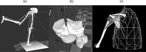
Data Collection. A constant challenge for the experimental motion analyst is the collection of accurate spatial displacement kinematics of a joint. Several methods have been employed. A review is presented here.
Video and digital optical motion capture (tracking) systems offer state-of-the-art, high resolution, accurate motion capture options to acquire, analyze, and display 3D motion data. The systems are integrated with analog
208 JOINTS, BIOMECHANICS OF
data acquisition systems to enable simultaneous acquisition (1–300 Hz) of force plate and electromyographic data. Clinically validated software analysis packages are used to analyze and display kinematic, kinetic, and electromyographic data in forms that are easy to interpret.
The major components of a video and digital motion capture system are the cameras, the controlling hardware modules, the software to analyze and present the data, and the host computer to run the software. These systems are designed to be flexible, expandable (from 3 to up to 200 cameras in motion analysis tracking for Hollywood animation movies) and easy to integrate into any working environment. This system collects and processes coordinate data in the least amount of time and requires minimal operator intervention. This system uses motion capture cameras to rapidly acquire 3D coordinate positions from reflective markers placed on subjects. Illuminating strobes with differing wavelengths are used to track the spatial displacement (between 1 and 10 mm resolution) of spherical reflective markers attached to the subject’s skin at appropriately chosen locations, preferably on bony landmarks on the human body to minimize skin movement. They can be infrared (IR), visible red, or near-IR strobes to fit the lighting conditions of the capture environment. Also, the lenses can be of fixed or variable focal length for total adaptability. Images are processed within the optical capture cameras where markers are identified and coordinates are calculated before being transferred to the computers. After the completion of the movement, the system provides 3D coordinate and kinematic data. The disadvantages of the system include the skin movement error whose effect is more prominent (3 cm error) at high movement speeds. These high speed motion tasks (impact biomechanics, e.g.) are handled by high speed cine cameras with data acquisition rates several orders of magnitude greater than clinical motion analysis systems. The processing method that is almost real time uses combinations of skin markers (minimum three at each segment) to produce coordinate systems for each segment and eventually describe intersegmental relative motion or relate all the different segment motions to the laboratory fixed-coordinate system. Recently, methods employing clusters of markers have shown to somewhat reduce the skin marker artifact but are yet to be adopted in the clinical practice.
A more accurate method (<1 mm translation and up to 1000 Hz) is the cineradiographical method, which employs an X-ray machine and uses special cameras for capture of sequences of the digital radiographs. In addition to accuracy, these systems directly access the in vivo skeletal kinematics so that the resulting analysis can be directly related to bony landmarks. Radiation issues, magnification, and distortion factors are some drawbacks that can be overcome by appropriate image analysis techniques. This method is, however, prone to occlusion errors when two segments overlap and simultaneously cross the field of view of the X-ray source. Stereosystems with more than one X-ray sources can limit this artifact. A biplane radiographic system consists of two X-ray generators and two image intensifiers optically coupled to synchronized high speed video cameras that can be configured in a custom gantry to enable a variety of motion studies. The system
can be set up with various set-up modes (e.g., a 608 interbeam angle), an X-ray source to object distance of 1.3 m, and an object to intensifier distance of 0.5 m. Images are acquired with the generators in continuous radiographic mode (typically 100 mA, 90 kVp). The video cameras are electronically shuttered to reduce motion blur. Short (0.5 s) sequences are recorded to minimize radiation exposure. X-ray exposure and image acquisition are controlled by an electronic timer–sequencer to capture only the desired phase of movement.
CODA is an acronym of Cartesian Opto-electronic Dynamic Anthropometer, a name first coined in 1974 to give a working title to an early research instrument developed at Loughborough University, United Kingdom. The 3D capability is an intrinsic characteristic of the design of the sensor units, equivalent to but much more accurate than the stereoscopic depth perception in normal human vision. The system is precalibrated for 3D measurement, which means that the lightweight sensor can be set up at a new location in a matter of minutes, without the need to recalibrate using a space-frame. Each sensor unit must be independently capable of measuring the 3D coordinates of skin markers in real-time. As a consequence, there is great flexibility in the way the system can be operated. For example, a single sensor unit can be used to acquire 3D data in a wide variety of projects, such as unilateral gait. Up to six sensor units can be used together and placed around a capture volume to give ‘‘extra sets of eyes’’ and maximum redundancy of viewpoint. This enables the system to track 3608 movements that often occur in animation and sports applications. The calculation of the 3D coordinates of markers is done in real-time with an extremely low delay of 5 ms. Special versions of the system are available with latency shorter than 1 ms. This opens up many applications that require real-time feedback, such as research in neurophysiology and high quality virtual reality systems, as well as tightly coupled real-time animation. It is also possible to trigger external equipment using the real-time data. The automatic intrinsic identification of markers combined with processing of all 3D coordinates in real-time means that graphs and stick figures of the motion and many types of calculated data can be displayed on a computer screen during and immediately after the movement occurs. The data are also immediately stored to file on the hard drive.
A new concept in measuring movement disorders utilizes a unique miniature solid-state gyroscope, not to be confused with gravity sensitive accelerometers. The instrument is fixed with straps directly on the skin surface of the structure whose motion is of interest. It has been successfully used to quantify: tremor (resting, posture, kinetic), rapid pronation–supination of the hand, arm swing, lateral truncal sway, leg stride, spasticity (pendulum drop test), dyskinesia, and alternating dystonia. The system (Motus) senses rotational motion only and is ideal for quantifying human movement since most skeletal joints produce rotational motion. This disadvantage is outweighed by its miniature size that allows it to be of great value for certain types of studies. A different system (Gypsy Gyro) uses 18 small solid-state inertial sensors (gyros) to accurately measure the exact rotations of the actor’s bones in real-time for motion capture. The system can easily be worn beneath
normal clothing. With wireless range these systems–suits can be used to record up to 64 actors simultaneously.
Another concept for 3D motion analysis is the measurement system CMS10 (Zebris) designed as a compact device for everyday use. The measurement procedure is based on the travel time measurement of ultrasonic pulses that are emitted by miniature transmitters (markers placed on the skin) to the three microphones built into the compact device. A socket for the power pack (supplied with the device) as well as the interface to a computer are located on the back of the device. The evaluation and display of the measurement data are carried out in real-time. It is possible to use either a table clamp or a mobile floor stand with two joints to support the measurement system.
Data Analysis
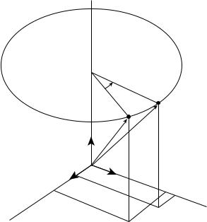
Coordinate Systems and Transformation. In the analysis of experimental joint mechanics data, the transformation of point coordinates from one coordinate system to another is a frequent task (4). A typical application of such a transformation would be gait analysis data recorded in a laboratory fixed coordinate system (by means of film or video sequences) that must be converted to a reference system fixed to the skeleton of the test subject. The laboratory fixed coordinate system may be designated by xyz and the body reference system by abc (Fig. 4). The location of a point S(a/b/c) in the body reference system is defined by the radius vector s ¼ a ea þ b eb þ c ec. Consider the reference system to be embedded into the laboratory system. Then the radius vector rm ¼ xm ex þ ym ey þ zm ez describes the origin of the reference system in the laboratory system. The location of S(x/y/z) is now expressed by the coordinates a, b, c. The vector equation r ¼ rm þ s gives the radius vector for point S in the laboratory system (Fig. 4). Employing the full notation we have: r ¼ ðx ex þ y eyþ
z ezÞ ¼ ðxm ex þ ym ey þ zm ezÞ þ ða ea þ b eb þ c ecÞ. A set of transformation equations results after some inter-
mediate matrix algebra to describe the coordinates. The scalar products of the unit vectors in the xyz and abc
ec
S
eb
S
ez r
ea
rm
ey
ex
Figure 4. Changing the coordinate systems, transformation of point coordinates from one coordinate system to another.
JOINTS, BIOMECHANICS OF |
209 |
R ′
t
R
t |
Q ′ |
Q
t
P ′
P
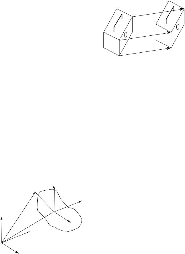
Figure 5. A rigid body (shoebox) moves parallel to itself. The radius vectors from O to P and from O to P0 are designated by r and r0 so that r0 ¼ r þ t, where t is the difference vector.
systems produce a set of nine coefficients Cij. The cosine of the angle between the coordinate axes of the two systems corresponds to the value of the scalar products. Three ‘‘direction cosines’’ define the orientation of each unit vector in one system with respect to the three unit vectors of the other system. Due to the inherent properties of orthogonality and unit length of the unit vectors, there are six constraints on the nine direction cosines, which leaves only three independent parameters describing the transformation. Employing the matrix notation of the
transformation equation we have |
|
|
|
||||||
x |
3 |
|
xm |
3 |
|
c11 c12 c13 |
3 |
a |
3 |
2y |
¼ |
2ym |
þ |
2c21 c22 c23 |
2b |
||||
6z |
7 |
6zm |
7 |
6c31 c32 c33 |
7 |
6c |
7 |
||
4 |
5 |
|
4 |
5 |
|
4 |
5 |
4 |
5 |
In coordinate transformations, the objects remain unchanged and only their location and orientation are described in a rotated and possibly translated coordinate system. If a measurement provides the relative spatial location and orientation of two-coordinate systems the relative translation of the two systems and the nine coefficients Cij can be calculated. The coefficients are adequate to describe the relative rotation between the two coordinate systems.
Translation in Three-Dimensional Space. In translation in 3D space, the rigid object moves parallel to itself (Fig. 5). Pure translation in 3D space leaves the orientation of the body unchanged as in the case of pure 2D translation.
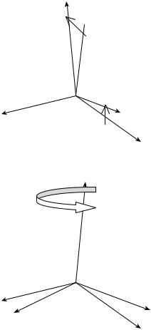
Rotations about the Coordinate Axes. A rotation in 3D space is defined by specifying an axis and an angle of rotation (Fig. 6). The axis can be described by its 3D orientation and location (5). A rotation, as does the translation explained earlier, leaves all the points on the axis unchanged; all other points move along circular arcs in planes oriented perpendicular to the axis (6,7).
This rotation moves an arbitrary point P to location P0 with constant distance z from the xy plane (z ¼ z0). This produces the following matrix notation for the respective equations for the rotation that changes x and y coordinates
210 JOINTS, BIOMECHANICS OF
|
|
g |
R |
|
|
|
|
|
|
|
|
P (x /y /z ) |
|
P ′(x ′/y ′/z ′) |
|
|
|
|
|
|
|
r |
r ′ |
|
ez |
|
ey |
z |
z′ |
|
||||
O |
|
|||
|
|
|
||
ex |
|
|
|
|
|
|
y ′ |
|
x |
y |
|
|
|
x ′ |
|
|
|
|
Figure 6. Rotation about the z axis of the coordinate system.
but leaves the z coordinate unchanged. |
3 |
|
||||||||
r0 |
|
2y0 |
3 |
|
2sing |
cosg |
0 |
32y |
Dz g r |
|
|
|
x0 |
|
|
cosg |
sing |
0 |
x |
|
|
|
¼ |
6z0 |
7 |
¼ |
60 |
|
1 |
76z |
7 |
¼ ð Þ |
|
0 |
|||||||||
|
|
4 |
5 |
|
4 |
|
|
54 |
5 |
|
The matrix describing a rotation about the z axis is designated Dz(l). The matrices describing a rotation about the y axis through angle b and about x axis through angle a are similar.
|
|
x |
3 |
|
2 |
cosb |
0 |
sinb |
|
|
x |
3 |
|
|
|
|
|
r0 |
¼ |
2y00 |
¼ |
0 |
sinb |
1 |
0 |
3 2y |
¼ |
Dy |
b |
r |
|||||
|
6z0 |
7 |
6 |
|
0 |
cosb |
7 |
|
6z |
7 |
ð |
Þ |
|
||||
|
|
4 |
5 |
|
4 |
|
|
|
5 |
|
4 |
5 |
|
|
|
|
|
r0 |
|
x |
3 |
|
2 |
1 |
0 |
0 |
x |
3 |
|
Dy a r |
|
2y00 |
|
0 |
cosa |
sina |
32y |
¼ |
|||||
|
¼ |
6z0 |
7 |
¼ |
6 |
0 |
sina |
|
76z |
7 |
ð Þ |
|
|
cosa |
|
||||||||||
|
|
4 |
5 |
|
4 |
|
|
|
54 |
5 |
|
|
Combined Rotations as a Result of a Sequence of Rotations.
Assume that the first rotation of a rigid body occurs about the z axis of a coordinate system. The rotation matrix related to the unit vectors ex, ey, ez, is
Dz |
g |
|
90 |
|
2 |
0 |
1 |
0 |
3 |
¼ |
Þ ¼ |
1 |
0 |
0 |
|||||
ð |
|
|
6 |
0 |
0 |
1 |
7 |
||
|
|
|
|
|
4 |
|
|
|
5 |
The second rotation occurs supposedly about the x0 axis, that is, about a body-fixed axis on the body (previously rotated about its z axis). The rotation matrix related to the unit vectors e0x, e0y, e0z, is
|
|
|
|
|
|
2 |
1 |
0 |
0 |
3 |
Dx0 |
ð |
a |
¼ |
90 |
Þ ¼ |
0 |
0 |
1 |
||
|
|
|
6 |
0 |
1 |
0 |
7 |
|||
|
|
|
|
|
|
4 |
|
|
|
5 |
Matrix intermediate calculation here gives
r00 ¼ Dz0 Dx0 r
In this calculation the sequence of the matrices is very important especially as this sequence differs from what one might expect. First, the matrix of the second partial rotation acts on the vector r and then, in a second step on the matrix of the first partial rotation. If the sequence of the two partial rotations is interchanged, the combined rotation is described by
r00 ¼ Dx Dz0 r
For rotations about body-fixed axes it is true that in general, the matrix of the last rotation in the sequence of rotations is the first one to be multiplied by the vector to be rotated. The matrix B describing the image resulting from n partial rotations about body-fixed axes is composed according to the formula:
Bbody - fixed ¼ D1 D2 D3 . . . Dn 1 Dn
where the indexes indicate the sequence of the rotations. Alternatively, if the n rotation were to be produced about axes fixed in space (i.e., fixed in the ground, laboratory frame) and not about body-fixed axes, the sequence of the matrexes in the matrix product would be different:
Bspace - fixed ¼ Dn Dn 1 . . . D2 D1
Euler and Bryant–Cardan Angles. Any desired orientation of a body can be obtained by performing rotations about three axes in sequence. There are, however, many ways of performing three such rotations. One can do this task at random, but for reasons of clarity two conventions are frequently used: the Euler’s and Bryant–Cardan’s rotations. In the Euler notation, the general rotation is decomposed of three rotations about body-fixed axes in the following manner:
Rotation 1: about the z axis through the angle w rotation matrix Dz(w) (Fig. 7).
Rotation 2: about the x0 axis through the angle u rotation matrix Dx0 ðuÞ.
Rotation 3: about the z00 axis through the angle c rotation matrix Dz00 ðcÞ.
The matrix describing Euler’s combined rotation is given by the matrix product
B |
¼ |
ð |
Þ |
ð Þ |
Dz00 |
ð |
Þ ð |
Euler |
Þ |
|
Dz |
w |
Dx0 u |
|
c |
|
According to the Bryant and Cardan the general rotation is decomposed of three rotations about body-fixed axes in the following manner:
Rotation 1: about the x axis through the angle w1 rotation matrix Dx(w1) (Fig. 7).
Rotation 2: about the y0 axis through the angle w2 rotation matrix Dy0 ðw2Þ.
Rotation 3: about the z00 axis through the angle w3 rotation matrix Dz00 ðw3Þ,
z′
 z
z
j1
x ′= x
y ′
y
z′ = z
x
j |
y ′ |
x ′
y
Figure 7. General rotation composed of three partial rotations. The first rotation according to the Bryant–Cardan convention (above). The first of the general rotations using Euler as the selection of the axes and angles of rotation (below).
in which case the matrix of combined rotation is given by
B ¼ Dxðw1Þ Dy0 ðw2Þ Dz00 ðw3Þ ðBryant CardanÞ
For reasons of simplicity, we have presented single or combined rotations about coordinate axes, but more complicated rotational laws can be applied as we deal with rotations about arbitrary axes. Rotation and translation can also be integrated into one single motion with Chasles theorem. Chasles theorem states that ‘‘the general motion in 3D space is helical motion’’, or ‘‘the basic type of motion adapted to describe any change of location and orientation in 3D space is helical motion’’. The relevant axis of rotation is designated the ‘‘helical axis’’. Chasles theorem is also known as the ‘‘helical axis’’ theorem.
KINETICS OF JOINTS
The study of the forces that bring about the movements discussed above is called kinetics. Because kinetics pro-
JOINTS, BIOMECHANICS OF |
211 |
vides insights into the cause of the observed motion, it is essential to the proper interpretation of human movement processes. Forces and loads are not visually observable; they must be either measured with instrumentation or calculated from kinematics data. Kinetic quantities studied include such parameters as the forces produced by muscles; reaction loads between body parts as well as their interactions with external surfaces; the load transmitted through the joints; the power transferred between body segments; and the mechanical energy of body segments. Inherent to such studies are the functional demands imposed on the body. The structure and stability of each extremity and its joints reflect different systems and functional demands. The functional demands on the upper extremity are quite different from those on either the upper and lower axial skeleton or those on the lower extremity. Depending on which joint and/or structure is addressed, different types and degrees of rotational motion are allowed and are functional. How much structural strength is needed versus how much movement is allowed in each area dictates the nature of the material, size, shape, and infrastructure of the joint system established to perform a given movement.
Equations of Motion
The kinetics deal with the effects of forces on the motion of a body. When the motion is known, the problem is then to find the force system acting on the body. There are joint forces and joint moments. With all the kinematic quantities known, it is possible to find the joint forces and moments from the resulting force system that acts on each element. This is done by solving a system of simultaneous equations at successive time intervals. Since muscles are an unknown force system, the resolved muscle force and the real joint force are treated as totally unknown joint forces in the analysis. The three equations of motion for linear motions are
X X X
F ¼ max F ¼ may F ¼ maz
The three equations of motion for rotation are
X
Mx ¼ Ixxax ðIyy IzzÞvyvz Ixyðay vxvzÞ
XIyzðv2y v2z Þ Ixxðaz þ vxvyÞ
|
My ¼ Iyyay ðIzz IxxÞvzvx Iyzðaz vyvxÞ |
X |
Ixxðvz2 vx2Þ Ixyðax þ vyvzÞ |
Mz ¼ Izzaz ðIxx IyyÞvxvy Izxðax vzvyÞ |
|
Ixyðvx2 vy2Þ Iyzðay þ vzvxÞ |
where M is the moment, I is the mass moment of inertia, a the angular acceleration, and v is the angular velocity. The moment equations can be simplified if the axes of the reference frames coincide with the principal axes, with the origin at the center of gravity. These equations, called Euler equations, are
X
XMx ¼ Ixax ðIy IzÞvyvz
XMy ¼ Iyay ðIz IxÞvzvx Mz ¼ Izaz ðIx IyÞvxvy
212 JOINTS, BIOMECHANICS OF
Continuity conditions are derived based on the fact that equal and opposite forces and moments occur at the joint between the two segments.
The anthropometric data for the mass, the center of gravity, the moment of inertia, and so on for the different parts of the human body are available in the literature (8,9).
Motion and Forces on Diarthroidal Joints
In vivo experimental measurements on the relative motions between articulating surfaces of a joint, which correspond to daily activities, are limited. Most quantitative information is obtained from gait studies that do not provide the accuracy and precision for the detailed information required for lubrication studies. However, even simple calculations show that translational speeds between two articulating surfaces can range from 0.06 m.s 1 between the femoral head surface and the acetabulum surface during normal walking, to 0.6 m.s 1 between the humeral head surface and the glenoid surface of the shoulder when a baseball pitcher throws a fastball. Cartilage to cartilage contact or fluid-film layers, or a mixture of both are normally the contact mechanisms at the joint. During a normal walking cycle, the human hip, knee, and ankle joints can be subjected to loads on the order of six times body weight, with these peak loads occurring just after heel-strike and just before toe-off. The average load on the joint is approximately three to five times body weight, which lasts as long as 60% of the walking cycle. During the swing phase of walking, only light loads are carried. During this phase, the articular surfaces move rapidly over each other. In addition, extremely high forces occur across the joints in the leg during jumping. Descending stairs can load the knee with up to 10 times body weight, suggesting that the load on the joint surface is dependent on the task performed, that is, the loading sites change drastically as the articulating surfaces move relative to each other.
MATHEMATICAL AND MECHANICAL MODELS OF JOINTS
Locomotion results from complex, high dimensional, nonlinear, dynamically coupled interactions between an organism and its environment. Simple models called templates have been and can be made to resolve the redundancy of multiple legs, joints, and muscles by seeking synergies and symmetries. The simplest model (least number of variables and parameters) that exhibits a targeted behavior is called a template (10). Templates can be used to test control strategies against empirical data. Templates must be based in more detailed morphological and physiological models to ask specific questions about multiple legs, the joint torques that actuate them, the recruitment of muscles that produce those torques and the neural networks that activate the ensemble. These more elaborate models are called anchors. They introduce representations of specific biological details of the organism. The control of slow, variable-frequency locomotion appears to be dominated by the nervous system, whereas during rapid, rhythmic locomotion, the control may reside more within the mechanical system. Anchored templates of many-legged, sprawled-postured animals may suggest that passive,
dynamic self-stabilization from a feedforward, tuned mechanical system can reject rapid perturbations and simplify control. Future progress would benefit from the creation of a field embracing comparative neuromechanics. Both templates and anchors are part of a system of mathematical and structural definitions and standard methods of description and dissemination of knowledge. In the next few sessions an attempt is made to describe some of those methods.
The human musculoskeletal system is often modeled by joining rigid links with continuous mass distribution. The joint may be of the revolute or spherical type, with restrictions consistent with body construction. Usually, the human segments form an open linkage.
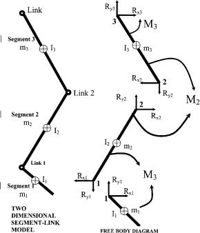
Knowing all the kinematics at the center of mass of the segments, the joint force and the moment analysis proceeds by drawing free-body diagrams of the segments involved. The free body diagrams for the hip joint, the knee joint, and the ankle joint in a sagittal plane are illustrated in Fig. 8 as an example:
Assessment of Mechanical Factors Associated With Joint Degeneration: Limitations and Future Work
Joint degeneration results from complex, multidimensional, nonlinear, dynamically coupled interactions between the organism and its environment. The assessment of mechanical factors associated with joint degeneration has traditionally combined longitudinal clinical studies with carefully designed experimental techniques and theoretical computational analyses. The quality of
Figure 8. Relationship between the free body diagram and the link-segment model. Each segment is ‘‘broken’’ at the joints, and the reaction forces and moments of force acting at each joint are shown.
such assessments depends both on the accuracy–precision of the measurement methodology and the theoretical framework for its interpretation (i.e. joint mathematical models). To capitalize on the increasing level of measurement accuracy, theoretical analysis requires more detailed morphological and physiological models (11). For example, because of variations between individuals, the detailed, morphological analysis required for accurate modeling of cartilage stresses must be patient specific. In addition, the dynamics of the human task to be modeled (for e.g., human jumping) as expressed in the strain rate of tissue deformation must be accounted for in the analysis. Once the error estimate (simulation versus experiment) is established, model predictions can address specific clinical-biological questions. Traditionally, in situ methodology (cadaveric experiments and in vitro tests) is applied when an in vivo measurement is impossible. This limitation presents a number of implications and assumptions that weaken the theoretical analysis. Recent developments have further improved accuracy in the experimental measurement of in vivo knee kinematics. These developments allow significant improvements upon previous limitations by applying patient-specific task-dependent models in the study of joint pathogenesis.
The vast majority of dynamic knee studies have been performed with conventional motion analysis techniques, using markers attached to the skin. Conventional motion analysis is not sufficiently accurate to enable analysis of cartilage stress. Previous studies have shown that skin markers move substantially relative to underlying bone, with RMS errors of 2–7 mm and peak errors as large as 14 mm in estimates of tibial position during gait (12). A study of four subjects during running and hopping (using 250 frame s 1 stereo radiography) has demonstrated skin marker motion relative to the femur averaging 1–5 mm throughout the motion, with peak-to-peak errors of the oscillation at impact averaging 7–14 mm (13). Errors were both subject and activity specific (14). Techniques have been developed for improving estimates of bone dynamics from skin markers using large numbers of markers and optimization–modeling of soft tissue deformation (15,16) but the performance of these methods for in vivo studies has only been validated for the tibia (during a slow, impactfree 10 cm step-up movement of a single patient with an external fixator). Average errors were low, but peak errors routinely exceeded 1 mm. Errors would likely increase significantly during faster movements and movements involving impact, and also where the soft tissue layer between skin and bone is thicker (e.g., for the femur). However, if the kinematic measurements are to be used in conjunction with musculoskeletal models to estimate dynamic loads and stresses on joint tissues, then even errors as small as 1 mm may be unacceptable. For example, when estimating strains in the ACL, a 1 mm error in tibio–femoral displacement could introduce uncertainty in the ligament length of approximately 3% (assuming a nominal ligament length of 30 mm). This error is similar in magnitude to estimated peak ligament elongation occurring during common activities, such as stair climbing (17). For investigating cartilage deformation, this error magnitude would be even less acceptable. A 1 mm displacement
JOINTS, BIOMECHANICS OF |
213 |
would be equivalent to a cartilage strain of 25%, relative to the average thickness of healthy tibio–femoral cartilage (18). A displacement error of this magnitude would translate into huge differences in estimates of contact forces. Thus, efforts to model, predict and correct for soft tissue deformation are unlikely to achieve sufficient accuracy for assessing soft tissue behavior. Alternatively, kinematics from a high speed stereoradiographic system capable of tracking implanted tantalum markers in vivo with 3D accuracy and precision better than 0.072 mm in translation and 0.358 in rotation (19) are more appropriate in use with advanced computational models. This accuracy is an order of magnitude or greater of improvement over conventional motion analysis techniques, and is uniquely capable of providing the accuracy necessary to model joint stresses.
From Experimental to Advanced Theoretical Analysis in Joint Mechanics
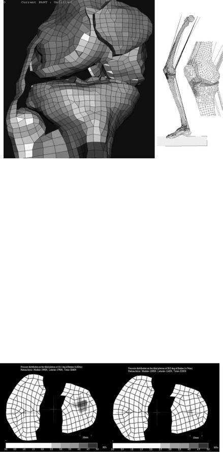
In addition to measuring joint kinematics and contact areas, investigators have attempted to measure articular contact stresses and pressures. However, stresses throughout the cartilage layer cannot be measured experimentally. Direct measurements of stress can be made at the articular surface using pressure sensing devices (20–22) (e.g., pressure sensitive Fuji film, piezoresistive contact pressure transducers, dye staining, silicone rubber casting). For cadaver studies, Fuji film sheets (Fuji Prescale Film; Itoh, New York, NY) are inserted in a joint and if pressed produce a stain whose intensity depends on the static applied pressure. Alternatively, digital electronic pressure sensors (e.g., K-scan, Tekscan, Boston, MA) can be placed onto the articular surface. These sensors are thin and flexible, and can be made to conform to the anatomy of the medial and lateral knee compartments. They consist of printed circuits divided into grids of load-sensing regions. Each load-sensing region within the grid has a piezoresistive pigment that can be used to determine the total compressive load within that region. After appropriate calibration procedures, dynamic pressure distributions can be calculated. In addition to providing a continuous, dynamic readout, K-scan has been reported to more accurately estimate contact areas than Fuji film (23,24).
There are significant concerns with the use of these sensors for estimating actual contact pressures. These techniques measure only surface-layer stresses, they alter the nature of cartilage surface interactions and are too invasive for in vivo human use. Thus, the clinical validity of articular pressure measurement with such sensors is questionable. They can, however, be important tools for the evaluation of the predictive power of joint models (2). By including the sensor in a finite element model, the effects of the sensor film on the actual contact mechanics can be accounted for (25). Thus, contact pressure predictions from such models can be directly compared to the pressure sensor measurements for finite element (FE) model validation.
Many in situ experimental studies have been conducted to obtain 3D knee joint kinematics and force-displacement data (21,26–30). Cadaver studies, however, cannot reproduce the complex loading seen by the joint during strenuous movements, since the muscle forces driving the
214 JOINTS, BIOMECHANICS OF
movement cannot be simulated. Because of these fundamental limitations of experimental measures, mathematical models are favored for obtaining comprehensive descriptions of the spatial and temporal variations of cartilage stresses. A numerical model could be used to perform parametric studies of geometry, loading or material properties in controlled ways that would not be possible with tissue samples.
Theoretical Analysis of Joint Mechanics
During the last two decades, a number of theoretical joint mechanics studies with different degrees of accuracy and predictive power have been presented in the literature (31– 39). Computational modeling work has included anatomical or geometrical observation (40,41) and analytical mathematical modeling (42–46). More recently, advanced FE modeling approaches allowed for improvements in the predictive power of localized tissue deformation (47–54). Joint biomechanics problems are characterized by moving contacts between two topologically complex soft tissue layers separated by a thin layer of non-Newtonian synovial fluid. A prime example is the multibody sliding contact problem between the tibia, femur, and menisci. The complexity of such problems requires implementation of sophisticated numerical methods for solutions (55–58). The finite element method is ideally suited for obtaining solutions to joint contact problems. Thus far, much of the finite element analysis has been applied to the study of hard tissue structures, often as it relates to prosthetic devices (59,60). When addressed, soft tissue layers are treated as single-phase elastic materials. As a consequence of the relative dearth of precise patient specific geometric data, material properties and insufficiency in accuracy of in vivo kinematics for input, no patient specific computational models have been reported for longitudinal clinical joint studies.
Surface Modeling
Surface modeling methods calculate the shape variations of joints and visualize the proximity of subchondral bone surfaces during static loading or dynamic movement. These methods can combine in situ data, motion analysis optical system data or high speed biplane radiographic image data and 3D bone surface information derived from computed tomography to determine subchondral bone motion. This method can be used to identify the regions of contact during static loading or dynamic motion, to calculate the surface area of subchondral bone within close contact, and to determine the changing position of the close contact area during dynamic activities (Fig. 9).
In vivo dynamic joint surface interaction information would be useful in the study of osteoarthritis changes in joint space and contact patterns over time, in biomechanical modeling to assist in finite element modeling, and in identifying normal and pathological joint mechanics preand postsurgery. Previous attempts to quantify the interaction between bones have utilized various methods including castings (62,63), pressure sensitive film (64), mathematical surface modeling (65,66), implant registra-
Figure 9. Example applications showing dynamic in vivo tibiofemoral bone surface motion using joint proximity (Euclidian distance) mapping during human one-legged hopping.
tion (67) and cine phase contrast magnetic resonance imaging (MRI) (68). The casting method can only be applied to cadaver models under static loading conditions. Pressure sensitive film also requires a cadaver model and necessitates inserting material into the joint space. Mathematical surface modeling allows analysis of dynamic motions in vivo, however, the joint must be disarticulated after testing. Implant registration requires either surgical implants or nonsubject specific image matching algorithms. Cine phase contrast MRI requires repeatedly performing the same motion pattern during testing and is limited to a small range of motion. The process described below is an improvement on these previous techniques because it utilizes live subjects performing dynamic tasks with unrestricted motion. Direct measurement of articular cartilage behavior in vivo during dynamic loading is problematic. In order to estimate the behavior of articular cartilage, the surface proximity interaction method that precisely tracks the motion of subchondral bone surfaces in vivo. Articular cartilage behavior is then estimated from these subchondral bone measurements.
Anderst et al. (61) described a method to estimate in vivo dynamic articular surface interaction by combining joint kinematics from high-speed biplane radiography with 3D bone shape information derived from computed tomography (CT). Markers implanted in the bones were visible in both the CT scans and the radiographic images, and were used to register the subchondral bone surfaces with the 3D bone motion. Joint surface interactions were then estimated by analyzing the relative proximity of the subchondral bone surfaces during the rendered movement. Computed Tomography data can be also used for joint geometry–shape characterization. The method is referred as reconstruction of volumetric models into rendered joint surface geometry models.
Computed Tomography data are typically collected for this method with slice spacing between the different images of 0.625 – 1.25 mm and the in-plane resolution
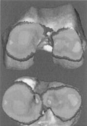
Figure 10. Articular surface matching (femoral condyle on top and tibial plateau below) using geometrical objects (69).
is 0.293–0.6 mm depending on the size of the bone. The CT scans are reconstructed into 3D solid figures using software that employs reconstruction techniques, that is, the regularized marching tetrahedra algorithm by Treece et al. (70). If necessary, threshold values are adjusted to ensure the entire bone surface appeared in the reconstruction and the opposing bone surfaces never overlapped in computer animations of the motion.
Anterior–posterior and lateral radiographs are commonly used to preoperatively determine prosthetic size and proper donor selection for osteochondral allografts. By using 3D computer aided design tools and the reconstructed 3D joint geometry from CT described above, size determination is less prone to out-of-plane imaging errors associated with sagittal and coronal roentgenograms. Assessment of surface size, curvature analysis and knee incongruity is possible with in vivo CT [Fig. 10 (69,71,72)]. After the 3D joint surface reconstruction models the distal articular femur (n ¼ 16) can be represented by six circles, the diameters of these circles, their angular arcs, and the distances between their centers varied with the size of the femur (Fig. 11; Table 5). There is a statistically significant association between several geometry parameters when the lateral or the medial distal femur is studied independently. These associations do not exist when we correlate medial versus lateral compartments across the population.
DA |
DP |
|
(b) |
||
|
||
|
DC |
X
Y
A
F E
Anterior
Posterior
Figure 11. All the sagittal view measured parameters in the study of femoral head congruity (69).
JOINTS, BIOMECHANICS OF |
215 |
The Joint Distribution Problem
Much attention has been devoted to the solution to what has become known as the general joint distribution problem that is, the problem of estimating the in vivo forces transmitted by the individual anatomical structures in the joint neighborhood during some activity of interest (73). The prediction of forces in joint structures has many applications. In the field of medicine, these predictions are useful for obtaining a better understanding of muscle and ligament function, mechanical environment within which prosthetic components must operate, and mechanical effects of musculoskeletal diseases. In the realm of sport biomechanics, these predictions are useful for better understanding of the kinetic demands, performance constraints, and mechanisms for improving athletic performance. Industrial applications include the optimization of occupational performance and safety considerations. Although the general techniques for predicting forces in joint structures may be used throughout this broad range of applications, the particular method of choice and the details of the analysis depend on the application.
The general force distribution problem normally arises in the following way. The musculoskeletal system or a relevant portion thereof is modeled as a mechanical system consisting of a number of essentially rigid elements (body segments) subjected to forces due to the presence of a gravitational field, and segmental contact with external objects, neighboring segments, and soft tissue structures that produce and constrain system motion. The associated inverse dynamics problem is then formulated and solved to determine the variable intersegmental (joint) force and moment resultants during the activity of interest. The joint resultants are abstract kinetic quantities that represent the net effect of all the forces transmitted by the anatomic structures crossing the joint. At a typical joint, these forces normally include the forces transmitted by the muscles, ligaments, and articular (bony) contact surfaces.
The unknown forces transmitted by the joint structure are next related to the known intersegmental resultants by writing the joint equilibrium equations. These equations express the fact that the vector sum of all the forces in the individual anatomic structures, and the vector sum of all the moments about the joint center produced by those forces, are equal to the intersegmental resultant force and moment, respectively. Assuming that all joint geometry (point of application and orientation of forces) is known and that these two independent vector equations (or six independent scalar equations) involve as unknowns the M muscle and L ligament forces, together with the 3C scalar components of the C bony contact forces, these joint equilibrium equations are indeterminate whenever the sum (M þ L þ 3C) of the unknown forces exceeds six. Thus, if the system model includes only one bony contact force (C ¼ 1) and more than three muscle and/or ligament forces (M þ L > 3), the corresponding joint distribution problem will be indeterminate and therefore have an infinite number of solutions.
Finally, the joint resultants are decomposed or distributed to the individual joint structures at each instant of