282 LUNG SOUNDS

characteristics. This may allow noninvasive monitoring of conditions such as pneumonia, congestive heart failure, or pleural effusion that increase intrathoracic density. Chronic obstructive lung disease may be detected by reading lung sound maps showing time intensity plots at several sites over the chest; this appears to be more accurate than current clinical diagnostic methods. The ability to detect diaphragmatic movement by multichannel lung sound analysis suggests that it may prove to be an inexpensive bedside test. It may also have useful applications in ventilator management.

It seems clear that wider application of these new developments in lung sound analysis will lead to safe, useful, and rewarding forms of clinical and physiological information that can answer many imaging, diagnostic, and monitoring problems.

BIBLIOGRAPHY

1.Laennec RTH. De l’auscultation mediate ou traite du diagnostic des maladies des poumon et du coeur, fonde principalement sur ce nouveau moyen d’exploration. 1st French ed., Volumes 2, Paris: Brosson et Chaude; 1819.

2.Laennec RTH, trans. by Forbes J 1st American ed. Philadelphia: James Webster; 1823. p 211.

3.Mikami R, Murao M, Cugell DW, Chretien J, Cole P, MeierSydow J, Murphy RL, Loudon RG. International symposium on lung sounds. Synopsis of proceedings. Chest 1987;92:342–345.

4.Bettencourt PE, Del Bono EA, Spiegelman D, Herzmark E, Murphy RL. Clinical utility of chest auscultation in common pulmonary diseases. Am J Respir Crit Care Med 1994;150: 1291–1297.

5.Pasterkamp H, Kraman SS, Wodicka GR. Respiratory sounds. Advances beyond the stethoscope. Am J Respir Crit Care Med 1997;156:974–987.

6.Sovijarvi AHA, Vanderschoot J, Earis JE. Computerized Respiratory Sound Analysis (CORSA): Recommended standards for terms and techniques. Eur Respir Rev 2000;10: 77:585–649.

7.Sakula A. Laennec RTH 1781–1926. His life and work. A bicentenary appreciation. Thorax 1981;36:81.

8.Ertel PY. Stethoscope acoustics and the engineer: Concepts and problems. J Audio Eng Soc 1971;19:182–188.

9.Charbonneau G, Sudraud M. Measurement of the frequency response of some commonly used stethoscopes. Consequences to cardiac and pulmonary auscultation. Bull Eur Physiol 1985;21:49–55.

10.Abella M, Formolo J, Penney DG. Comparison of the acoustic properties of six popular stethoscopes. J Acoust Soc Am 1992;91:2224–2228.

11.Charbonneau G, Racineux JL, Sudraud M, Tuchais E. An accurate recording system and its use in breath sounds spectral analysis. J Appl Physiol 1983;55:1120–1127.

12.Pasterkamp H, Kraman SS, DeFrain PD, Wodika GR. Measurement of respiratory acoustical signals. Comparison of sensors. Chest 1993;104:1518–1993.

13.Kraman SS. Lung sounds: Relative sites of origin and comparative amplitude in normal subjects. Lung 1983;161:57–64.

14.Pasterkamp H, Fenton R, Tal A, Chernick V. Interference of cardiovascular sounds with phonopneumography in children. Am Rev Respir Dis 1985;131:61–64.

15.Kraman SS, Wodicka GR, Oh Y, Pasterkamp H. Measurement of respiratory acoustic signals. Effect of microphone air cavity width, shape, and venting. Chest 1995;108:1004–1008.

16.Cugell DW. Use of tape recordings of respiratory sound and breathing pattern for instruction in pulmonary auscultation. Am Rev Respir Dis 1971;104:948–950.

17.Banaszak EF, Kory RC, Snider GL. Phonopneumography. Am Rev Respir Dis 1973;107:449–455.

18.Kompis M, Pasterkamp H, Wodicka GR. Acoustic imaging of the human chest. Chest 2001;120:1309–1321.

19.Sun X, Cheetam BM, Earis JE. Real time analysis of lung sounds. Technol Health Care 1998;6:11–22.

20.Bergstresser T, Ofengeim D, Vyshedskiy A, Shane J, Murphy

R.Sound transmission in the lung as a function of lung volume. J Appl Physiol 2002;93:667–674.

21.Fitzpatrick MF, Martin K, Fossey E, Shapiro CM, Elton RA, Douglas NJ. Snoring, asthma and sleep disturbance in Britain: a community-based survey. Eur Respir J 1993;6:531–535.

22.Dalmasso F, Prota R. Snoring: analysis, measurement, clinical implications and applications. Eur Respir J 1996;9:146–159.

23.Kraman SS, Wodicka GR, Kiyokawa H, Pasterkamp H. Are minidisc recorders adequate for the study of respiratory sounds?. Biomed Instrum Technol 2002;36:177–182.

24.Krumpe PE, Hadley J, Marcum RA. Evaluation of bronchial air leaks by auscultation and phonopneumography. Chest 1984;85:777–781.

25.Ploysongsang Y, Martin RR, Ross RD, Loudon RG, Macklem PT. Breath sounds and regional ventilation. Am Rev Respir Dis 1977;116:187–199.

26.McKusick VA, Jenkins JT, Webb GN. The acoustic basis of the chest examination: Studies by means of sound spectrography. Am Rev Tuberc 1955;72:122–134.

27.Murphy RLH, Holford SK, Knowler WC. Visual lung sound characterization by time-expanded wave-form analysis. N Engl J Med 1977;296:968–971.

28.Baughman RP, Loudon RG. Lung sound analysis for continuous evaluation of airflow obstruction in asthma. Chest 1985;88:364–368.

29.Pasterkamp H, Tal H, Leahy F, Fenton R, Chernik V. The effect of anticholinergic treatment on post exertional wheezing in asthma studied by phonopneumography and spirometry. Am Rev Respir Dis 1985;132:16–21.

30.Nath AR, Capel LH. Inspiratory crackles and the mechanical events of breathing. Thorax 1974;29:695–698.

31.Murphy RLH, Jr., Gaensler EA, Holford SK, Delbono EA, Eppler G. Crackles in the early detection of asbestosis. Am Rev Respir Dis 1984;129:375–379.

32.Kiyokawa H, Pasterkamp H. Volume-dependent variations of regional lung sound, amplitude, and phase. J Appl Physiol 2002;93:1030–1038.

33.Que C-L, Kolmaga C, Durand L-G, Kelly SM, Macklem PT. Phonospirometry for noninvasive measurement of ventilation: Methodology and preliminary results.J Appl Physiol 2002;93:1515–1526.

34.Bergstresser T, Ofengeim D, Vyshedskiy A, Shane J, Murphy

R.Sound transmission in the lung as a function of lung volume. J Appl Physiol 2002;93:667–674.

35.Paciej R, Vyshedskiy A, Shane J, Murphy R. Transpulmonary speed of sound input into the supraclavicular space. J Appl Physiol 2002;94:604–611.

36.Winchester JF, Tohme WG, Schulman KA, Collman J, Johnson A, Meissner MC, Rathore S, Khanafer N, Eisenberg JM, Mun SK. Hemodialysis patient management by telemedicine: Design and implementation. ASAIO J 1997;43:M763–766.

See also PULMONARY PHYSIOLOGY; RESPIRATORY MECHANICS AND GAS EXCHANGE.

LVDT. See LINEAR VARIABLE DIFFERENTIAL TRANSFORMERS.

M

MAB. See MONOCLONAL ANTIBODIES.

MAGNETIC RESONANCE IMAGING

W. F. BLOCK

A. L. ALEXANDER

S. B. FAIN

M. E. MEYEREND

C. J. MORAN

S. B REEDER

K. K. VIGEN

O. WIEBEN

University of

Wisconsin–Madison

Milwaukee

Madison, Wisconsin

J. H. BRITTAIN

General Electric Healthcare

Milwaukee, Wisconsin

INTRODUCTION

The principle of nuclear magnetic resonance (NMR) was discovered by Felix Bloch and Edward Purcell independently in 1946. The two were awarded the Nobel Prize in Physics for the discovery, which had numerous applications in studying molecular structure and diffusion. Atomic nuclei with an odd number of protons or an odd number of neutrons behave like spinning particles, which, in turn, create a small nuclear spin angular momentum. This angular momentum of an electrically charged particle such as the nucleus of a proton leads to a magnetic dipole moment. In the absence of an external magnetic field, the orientation of these magnetic moments is random due to thermal random motion. These magnetic moments are referred to as spins, because the fundamentals of the phenomena can be explained using classical physics where the moments act similarly to toy tops or gyroscopes. The NMR phenomenon exists in several atoms and is used today to study metabolism via imaging. However, hydrogen is the simplest and most imaged nucleus in MR examinations of biological tissues because of its prevalence and high signal compared with other nuclei.

NMR imaging was renamed Magnetic resonance imaging (MRI) to remove the word nuclear, which the general public associated with ionizing radiation. MRI can be explained as the interaction of spins with three magnetic fields: a large static field referred to as B0, which organizes the orientation of the spins; a radio frequency (RF) magnetic field referred to as B1, which perturbs the spins so that a signal can be created; and spatially varying magnetic fields referred to as gradients, which encode the spatial location of the spins. These subsystems are shown in Fig. 1.

When an external magnetic field is present, the distribution of the magnetic moments is no longer random. Current technology allows large, homogenous static

magnetic fields to be created using superconducting magnets, whereas smaller fields are possible with permanent magnets. In most conventional systems, the static field is aligned along the longitudinal axis or the long axis of the body, as shown in the z axis in Fig. 1. Clinical MRI scanners have been built with static fields ranging from 0.1 to 7 T, but the vast majority of scanners are between 0.5 and 3.0 T.

THEORY

Creating Net Magnetization

Consider a static field oriented along the z axis with magnitude B0, or represented as a vector B ¼ B0k. Hydrogen protons have a quantum operator whose z component is quantized to ½. According to quantum mechanics, only two discrete sets of orientations exist for the magnetic dipole of each hydrogen nucleus. In the parallel energy state, the magnetic moment vector m orients itself so that its projection on the z axis aligns with the direction of the main magnetic field B0. In the antiparallel energy state, this projection aligns in the opposite direction of the main field. It can be shown that the two allowed angles between magnetic dipoles and the static field are u ¼ 548 (1), and thus a population of spins will be oriented as in Fig. 2b.

The ratio of spins in the parallel state n to the spins in antiparallel state nþ is given by the Boltzmann equation

n DE		¼ e	g2pB kT
	¼ e kT		h 0	(1)
nþ

where g is a nuclei-specific constant referred to as the gyromagnetic ratio, k denotes the Boltzmann constant, and T is the absolute temperature. There are only slightly more spins in the parallel state than in the antiparallel state because this state is of lower energy; however, the prevalence of water in biological tissue can create an adequate signal with this differential. This distribution of spin orientations in a small volume element results in an average or net magnetization M, which aligns along the longitudinal or z axis, as shown in Fig. 2b. The entire process is referred to as polarization. The contributions in the transverse (x y) plane sum to zero. As the argument of the exponential in Equation 1 is small and the difference in energy levels varies proportionally with field strength, the length of the net magnetization vector varies linearly with field strength. A quantum mechanics description of the spin distribution can be found elsewhere (2).

Signal Generation

The behavior of the net magnetization vector in an external field can be described by the classical model according to

283

284 MAGNETIC RESONANCE IMAGING

Figure 1. Clinical 1.5 T MRI scanner with static field oriented along long axis of the body (z). Patient’s head lies in RF coil, which is used to both perturb and receive MR signal. Scanner bed will move patient into middle of cylinder before imaging begins. MR gradient coils for y dimension are shown, which have mirrored coils on the opposite side of the magnet. A portion of the z gradient, based on solenoid design, is also shown.

Superconducting magnet

Y gradient coil

	y
z	x
	RF Transmitter and Receiver
B0	Z gradient coil

the Bloch equation.

dM	¼ gðM BÞ	(2)
dt

A useful parallel description is a spinning toy top where the axis of the top is analogous to M and gravity is analogous to B. In the equilibrium state, the net magnetization M and the static magnetic field B0 are parallel so that M does not experience a torque and consequently the direction of M does not change. Similarly, the axis of a spinning top oriented vertically remains vertical.

The second magnetic field in MRI is an RF field that is created using an RF amplifier that supplies oscillating current into a coil that surrounds the patient. The coil is designed to create a magnetic field, referred to as B1 field, oriented in the transverse plane and approximately on the order of 10 T. By having the RFenergy oscillate at the resonant frequency of the nuclei, this relatively low field can perturb and rotate the net magnetization away from its orientation along the longitudinal axis. The resonant or Larmor frequency v0 is related to the static field strength such that v0 ¼ gB0. For protons, the gyromagnetic ratio g/2p ¼ 42.57 MHz/T. The field created by the tuned RF coil, referred to as an excitation, can be

viewed as an applied torque that tips or flips spins away from the longitudinal axis by an angle referred to as the flip angle. The strength of the B1 field and the length of time it is applied determine the flip angle. The flip angle usually varies between 5 and 1808 depending on the application.

Once the magnetization is no longer parallel to the static field, the right-hand side of Equation 5 is no longer zero and the direction of the net magnetization will change. In fact, it will begin to precess about the axis of the static magnetic field and at the Larmor frequency. In general, the precessional frequency is directly proportional to the magnetic field experienced by the spin, such that v ¼ gB. Similar to a toy top that is tipped an angle u off its vertical axis, the top will maintain an angle of u as it rotates about the vertical force supplied by gravity.

The net magnetization can be described by its longitudinal component Mz and its transverse component Mxy, a complex value whose magnitude describes the component’s strength and whose angle describes the location of the component in the x–y plane. The rapid rotation of the transverse component will create a time-varying magnetic flux. A properly oriented receiver coil will detect this timevarying flux as a time-varying voltage, in agreement with Faraday’s law of induction. Often, the same coil used for excitation can also be used for reception. This voltage signal, known as a Free Induction Decay, or FID, is shown after a 908 excitation in Fig. 3, which is the most basic form of a MR signal. Although the entire magnetization vector is tipped into the transverse plane in this example, smaller flip angles will also create a transverse magnetization and thus an FID.

Figure 2. (a) shows the precession of a spin with a magnetic moment m in a static field with magnetic flux density of B0. An assembly of spins in parallel and antiparallel states is shown in (b). The Boltzmann equation determines the ratio of the spins in the two states. As the components in x and y compensate each other, the net magnetization M has a component in the z direction only (parallel to B0). The coordinate system is shown with its unit vectors i, j, and k along x, y, and z.

Figure 3. Generation of a free induction decay after a 908 RF excitation.

The complex motion of the net magnetization, and thus the recorded FID signal, can be described in a simplified manner by using a rotating reference frame that rotates at the Larmor frequency about the static B0 field. In this rotating frame, the FID will decay as a simple exponential. The causes of this decay, and its use as potential image contrast mechanism, will be described after spatial encoding is described. Most MR signals are demodulating using the Larmor frequency and, thus are effectively acquired in the rotating frame.

Spatial Encoding

The first two magnetic fields described above allow biological tissue to be polarized, perturbed, and measured. In terms of clinical imaging, however, these fields merely allow us to integrate the signal derived throughout the body, a measure of little value. The field of MRI developed only when a third spatially varying magnetic field, referred to as a gradient field, was invented to spatially encode the MRI signal. This method allows us to achieve submillimeter resolution while using RF energy whose wavelengths are on the order of tens of centimeters to meters.

Dr. Paul Lauterbur realized, in 1973, that, instead of working like others to build a more homogenous field for NMR spectroscopy, spatially varying the strength of the magnetic field could provide a means to build an imaging system. For this work, he won the Nobel Prize in Medicine along with Sir Peter Mansfield in 2003.

The three gradient coils in a cylindrical MRI system, two of which are shown in Fig. 1, are laid out concentrically on a cylinder. The cylinder surrounds the patient as he or she lies inside of the static B0 field. The three coils are designed to create longitudinal magnetic fields in z that vary in strength linearly with the x, y, and z dimensions, respectively. The digital scanner hardware controls the current waveforms, which are amplified by three respective gradient amplifiers before being sent to the gradient coils. The strength of each component gradient field, Gx,Gy, or Gz, is measured in G/cm or mT/m and is directly proportional to the current supplied to the coil. Changing gradient strengths quickly on clinical scanners is possible with amplifiers capable of slew rates of approximately 200 mT/m/s.

As the resonant frequency of an MR spin is directly proportional to the magnetic field it experiences, a gradient coil allows us to linearly vary the frequency of spins according to their position within the magnet. For example, a gradient of strength Gx, which does not vary in time, causes the frequency of spins to vary linearly with the x

coordinate.
wðxÞ ¼ g½B0 þ Gxx&	ð3Þ

Spins to the left of the magnet center rotate slower, spins at the exact magnet center remain unchanged, and spins to the right rotate faster than they did without the gradient.

Gradients can be used to selectively excite only spins from a slice or slab of tissue. Slice thicknesses in 2D MRI range from 1 to 20 mm. To select a transverse slice, the z gradient can be applied during RF excitation, which will cause the resonant frequency to vary as a function of z in

MAGNETIC RESONANCE IMAGING

285

the magnet, such that wðzÞ ¼ g½B0 þ Gzz&. Instead of exciting all the spins within the magnet, only spins whose frequency matches the narrow bandwidth of a pulsedRF excitation will be excited within a slice at the center of the magnet. Modulating the frequency of the RF pulse up will move the slice superior in the body, whereas modulating it down will excite an inferior slice. Likewise, slices perpendicular to the x or y axis can be excited by applying a Gx or Gy gradient, respectively, simultaneously with RF excitation. In fact, an oblique slice orientation can be achieved with a combination of two or more gradients. The ability to control from which tissue signal is obtained, without any patient movement, is a major advantage of MRI.

Simplified MR Spatial Encoding. Once a slice of tissue is selected, the two remaining spatial dimensions must be encoded. A somewhat simplified method of visualizing encoding follows. For a transverse slice, receiver data could be obtained after RF excitation while a constant gradient was applied in the x direction. Tuning a receiver to select a very narrowband frequency range would determine which spins were present within a spatial range x1< x< x1 þ Dx. By repeating the experiment while changing the narrowband frequency range, a projection of the spin densities along the x axis could be determined. Likewise, the same experiment could be repeated while applying a constant y gradient to obtain a projection of spin densities along the y axis. Likewise, projections along arbitrary axes could be achieved by acquiring data while applying a combination of x and y gradients after RF excitation. In a matter very similar to computed tomography (CT) imaging, an image could be reconstructed from this set of acquired projections.

MR Spatial Encoding in the Fourier Domain. Although possible, the proposed method would be very slow because each sample point within each projection would require its own MR experiment or excitation. Time between excitations in MR vary in duration from 2 ms to 4 s depending on the desired image contrast. Even with the shortest excitation, each slice would require over 3 min of scan time. All the data for an entire projection can be acquired within milliseconds by considering how the phase of the transverse magnetization varies, instead of the frequency, with spatial position. This description also uses the concept that position in MR is encoding using an alternative Fourier domain where signal location is mapped onto spatial frequencies.

Integrating the frequency expression in Equation 3 indicates how the spin phase, or location of the transverse magnetization within the transverse plane, will vary with the x coordinate during a general time-varying gradient Gx(t) applied after excitation. Ignoring the phase term due to the B0 field, which will be removed during demodulation of the received signal, gives a phase term for each spin that varies with the spatial position x and the integral of the applied gradient at each point in time.

		g	t
	Mxyðx; tÞ ¼ MxyðxÞe j2 p		R t0¼0	½Gxðt0Þx&dt0	(4)
		2p

286 MAGNETIC RESONANCE IMAGING

The signal received by the MR coil can be expressed as an integration of all the excited spins in the x–y plane using the following equation:

Z Z

SðtÞ ¼ Mxyðx; yÞe j2pkxðtÞxdx dy (5)

y x

where a Fourier spatial frequency, termed kx(t) in MR, has

	2p			t0	¼o	ð		ð		Þ Þ
been substituted for		g		t			Gx		t0	x dt0. In this example,
the coil simply	integrates all the spins in the y dimension,
			R

and thus only spatial information in x is available. The received signal can be seen as a 1D Fourier transform of the projection of transverse magnetization Mxy(x, y) onto the x axis. The corresponding coordinate in the Fourier domain at each point in time t is determined by the ongoing integral of the gradient strength. Thus, we can acquire an entire projection in one experiment rather than numerous MR experiments as in the simplified example with the narrowband receiver.

The last spatial dimension for this 2D imaging example y has a corresponding Fourier dimension termed ky, which can be similarly traversed by designing the integral of the Gy gradient current.

SðtÞ ¼ Zy		Zx	Mxyðx; tÞe j2pkxðtÞx e j2pkyðtÞydxdy		(6)
where kyðtÞ ¼	g		t	ðGxðt0ÞxÞdt0. The integral of the gra-
	2p		t0¼o

R

dients determines location in the Fourier space known as k space in MRI. Numerous strategies can be used to traverse and sample k space before transforming the data, often with a Fast Fourier Transform (FFT), into the image domain. The method can be extended to three dimensions by exciting a slab of tissue and using the Gz gradient to encode the third dimension.

As in the simplified example, a combination of Gx and Gy can be used to sample the 1D Fourier expression of projections of Mxy at arbitrary angles. This data can be transformed into the actual projections using 1D inverse Fourier transforms. Methods very similar to computed tomography can translate the projection data into an image. Although acquiring data in this manner, known as radial imaging, has interesting properties, by far the most popular method in clinical imaging traverses the Fourier space in a Cartesian raster pattern known as spin-warp imaging.

This sampling is typically completed	in a series
of experiments, where the time between	consecutive

excitations is referred to as the repetition time TR. In many MR acquisition schemes, a complete k space line is acquired along kx, known as the frequency-encoding or readout direction, for each TR. During each subsequent TR, a line parallel to the previous one is sampled after applying a short, pulsed Gy gradient. By changing the strength of the pulsed Gy gradient by equal increments during each MR experiment, a different phase shift is placed on spins depending on their position in y. In terms of the k space formalism, the area under the Gy gradient pulse causes a vertical displacement in k space such that a different horizontal line in k space is acquired in each MR experiment, as shown in Fig. 4. Here, the vertical direction in k space is known as the phase-encoding direction. By applying 1D Fourier transforms in the kx direction, spin position is resolved based on their frequency during readout. An image is formed by following these horizontal transforms with 1D Fourier transforms in the ky dimension. Here, the y position of spins is resolved due to the different phase shifts experienced in each experiment prior to the readout gradient.

The image coverage, or field of view, in MRI decreases as the sampling rate decreases. As MR samples in the frequency domain, failure to sample fast enough in k space leads to aliasing in the image domain. Higher resolution in MRI requires obtaining higher spatial frequencies or larger extents of k space. Achieving adequate resolution and coverage then increases the amount of k space sampling that is required and increases imaging time. Unlike other modalities where hundreds to thousands of detectors can be used at a time, encoding spatial position in this method only allows one point of data to be taken at a time, which explains MR’s relatively slow acquisition speed. Industrial scanners have only recently determined how to partially bypass this limitation by using up to 32 different receivers who have different spatial sensitivities to different tissues. The differences of each receiver in proximity, and thus sensitivity to each spin, can be used to synthesize unacquired regions of k space.

Image Contrast Through Varying Decay Rates

Imaging the spatial density distribution of hydrogen often produces a very low contrast image, as the density of hydrogen is relatively consistent in soft tissue. However, the imaging experiments described above can be easily modified to exploit the differences in time for which the

Figure 4. 2D spin-warp imaging with one readout per TR. One complete line is sampled along the readout direction on a rectilinear grid in the Fourier domain (k space) with a resolution of Dkx (circles on the arrow). The next line is acquired parallel at a distance of Dky on the grid by increasing the phase-encoding gradient. This scheme is repeated until the desired grid is sampled. Images are reconstructed by an inverse 2D Fourier transform (FT).

MAGNETIC RESONANCE IMAGING

287

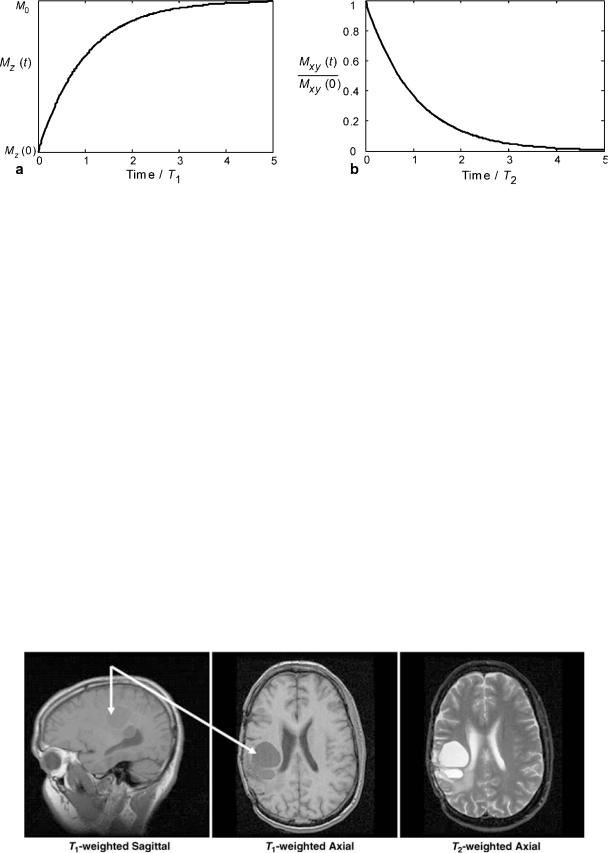
Figure 5. The regrowth of the longitudinal magnetization Mz (a) and the decay of the transverse magnetization Mxy (b) after an RF excitation.

MR spins remain perturbed. The differences account for the vast majority of image contrast in standard clinical MRI.

After the spins are perturbed, the transverse magnetization decays toward zero, whereas, the longitudinal magnetization returns toward its equilibrium magnetization. As more mechanisms exist for the loss of transverse magnetization than for the regrowth of longitudinal magnetization, the length of the magnetization vector M does not remain constant after excitation. Although related, the rate of longitudinal relaxation time, termed T1, is always larger than the rate of transverse relaxation time, termed

T2.

If the magnetization has been completely tipped in the transverse plane with a flip angle of 908, then the longitudinal magnetization recovers as

Mz ¼ M0½1 e t=T1 &

(7)

T1 is also called the spin–lattice relaxation time, because it depends on the properties of the nucleus and its interactions with its local environment. The transverse relaxation time T2 is also referred to as the spin–spin relaxation time, reflecting dephasing due to interactions between

neighboring nuclei.

Mxy ¼ Mxyð0Þe t=T2

(8)

where Mxy(0) is the initial transverse magnetization (Mxy(0) ¼ M0 for a 908 pulse). The temporal evolution of the longitudinal and transverse magnetization is shown in Fig. 5. In general, hydrogen protons in close proximity to macromolecules have lower relaxation times than bulk water that is freer to rotate and translate its position.

Delaying the encoding and acquisition of the transverse magnetization until some time after RF excitation generates T2 image contrast. As injured and pathological tissues generally have higher T2 relaxation rates, T2-weighted images have positive image contrast. T1-weighting can be achieved by using an interval between MR experiments, the TR parameter, which does not allow enough time for tissue to fully recover its longitudinal magnetization. Thus, tissues with shorter T1 relaxation rates will recover more quickly and thus have more signal present in the subsequent experiments used to build the image than tissues with longer T1. In general, T1-weighting provides negative contrast for pathological tissue. An example is shown in Fig. 6 for a human brain tumor. The differing rates of

Figure 6. The flexibility of MR to image in different planes with different types of image contrast is shown in these sagittal and axial brain tumor (arrows) images.

288 MAGNETIC RESONANCE IMAGING

Table 1. Longitudinal (T1) and Transverse (T2) Proton Nuclear Magnetic Resonance Relaxation Times for Several Tissues and Blood at 1.5 T

Tissue	T1/ms	T2/ms
Gray brain matter (3)	950	100
White brain matter (3)	600	80
Cerebrospinal fluid (CSF) (3)	4500	2200
Muscle (3)	900	50
Fatty tissue (3)	250	60
Oxygenated blood	1200	220
De-oxygenated blood	1200	120

recovery can also be used to null out an unwanted tissue, such as fat, by inverting all the spins 1808 prior to imaging. As the point where unwanted tissue passes through the null of the recovery phase, an imaging experiment is begun. This technique is referred to as inversion recovery magnetization preparation or simply inversion recovery. Table 1 lists representative relaxation times for some tissues (3). Extensive reviews of the relaxations times (4) and methods for their measurement (3,4) are available.

Spin Echoes

Ideally, the transverse magnetization decays according to T2. However, the signal dephasing in the transverse plane is significantly accelerated by field inhomogeneities due to difference in magnetic susceptibility between tissue types or the presence of paramagnetic iron. The largest inhomogeneities occur at air/tissue interfaces, such as near the sinuses or near the diaphragm. These effects lead to different precession frequencies and loss of coherence that are described by a T2 relaxation time

1	1		1		(9)
	¼		þ
T		T2		T0
2			2

where T02 represents the decay due to the effects described above.

A method to reverse these often undesirable dephasing effects uses a 908 pulse followed by a 1808 spin refocusing pulse after a time delay td, as shown in Fig. 7b. The first pulse rotates the longitudinal magnetization into the transverse plane as in the case of the FID. Prior to the second pulse, the magnetization dephases in the transverse plane due to T2 effects, with some spins

Figure 7. Generation of a (a) free induction decay and (b) a spin echo. In (a), other local factors dephase signal faster according to a T2 decay rate. If a second RF pulse is applied at time td ¼ TE//2 to flip the magnetization by 1808, the spins will refocus and form an echo at TE ¼ 2td, which is only subject to T2 decay.

rotating faster than the Larmor frequency and others spinning slower. The second pulse flips all magnetic moments about an axis in the transverse plane, effectively inverting the phase accruals due to different rotational frequencies. Over the second interval td, the faster spins will catch up with the slower spins. As a result, a spin echo is said to form at the time 2td, also known as the echo time or TE time. The amplitude of the signal at time TE is only decreased due to T2 decay whereas the T2 effects have been reversed. A simplified pulse sequence for the generation of a spin echo is shown in Fig. 7b without the gradient waveforms necessary for spatial encoding.

Signal-to-Noise Ratios

Signal in MR is generally proportional to the number of nuclei and, thus, to the volume of the image voxel. Noise in MR is caused by the random fluctuations of electrons in the patient, and thus the source of noise is independent from the signal generating sources. The data acquisition system is designed such that the noise level from properly designed

MR electronics will be dominated by patient noise. Overall, p

SNR ¼ voxel volume total data sampling time.

Imaging Sequences

Ideally, all MRI would be performed with high spatial resolution, a high signal-to-noise ratio (SNR), ultrashort imaging time, and no artifacts. The difficulty in achieving all of these properties simultaneously has led to the development of many acquisition methods that differ in image contrast, acquisition speed, SNR, susceptibility to and type of artifacts, energy deposited in the imaged patient, and suppression of unwanted signal such as fat. Their corresponding images represent a combination of tissue-specific parameters T1, T2, proton density r, and scan-specific parameters such as repetition time (TR), echo time (TE), flip angle, field of view (FOV), spatial resolution, and magnetization preparation.

Gradient Recalled Echo (GRE) Imaging

Spin-echo imaging is desirable because signal voids due to magnetic field inhomogeneity are avoided that could mask pathological tissue or injury. Long repetition times, and thus long scan times, are necessary in spin-echo imaging to allow longitudinal magnetization to return after the relatively high flip angles used. Long scan times hinder the capture of dynamic processes such as the beating heart, cause discomfort to the patient, and limit the number of patients who can be imaged with this expensive resource. Thus, other methods of imaging have been developed. In gradient recalled echo (GRE) imaging, the echo is formed by dephasing and rephasing of the signal with gradient fields as shown in Fig. 8. In these diagrams, known as pulse sequence diagrams, plots of the time-varying gradient and RF waveforms are shown as function of time. Compared with the spin-echo sequences, gradient recalled echo imaging does not have a refocusing RF pulse. The absence of this pulse allows for a reduced minimal repetition time and echo time compared with spin-echo imaging, but the signal becomes susceptible to T2* decay rather than T2 decay.

Figure 8. Basic 2D gradient echo pulse sequence. First, the magnetization is tipped into the transverse plane by an angle a during the application of a slice select gradient Gz. Then, the gradients Gy and Gx are used for phase encoding and the readout gradient. An echo forms at t ¼ TE when the area under the readout gradient is zero. This experiment is then repeated every TR with a different phase encode.

After RF excitation, the signal is dephased along the readout direction x with a prewinding gradient lobe. The amplitude of this gradient is then inverted to rephase the spins. When the area under the readout gradient is zero, the trajectory passes through the origin of k space and the echo forms with maximum amplitude. During the prewinder along the x axis, a gradient in y is played out to produce y depending on phase shifts for phase encoding.

By using a flip angle less than 908, significant amounts of transverse magnetization are available without the need for long repetition times needed for recovering longitudinal magnetization. For example, after a single 308 excitation, the transverse magnetization contains sin(308) or one-half of the available magnetization. Meanwhile, the longitudinal magnetization still contains cos(308) or nearly 87% percent of the equilibrium magnetization. In fast GRE imaging, the repetition time is significantly reduced and generally less than the T2 values of biological tissues. Under this condition, the transverse magnetization from preceding RF pulses is not completely dephased and generally results in a complex superposition of echoes from multiple RF pulses. Under certain conditions, a steadystate can be reached from repetition to repetition for one or more components of the magnetization (6).

GRE sequences can be used to generate T1, T1/T2, T2, T2 , and proton density-weighted contrast, depending on the choice of TR, TE, the flip angle a, and the phase f of the RF pulse. By altering the phase of the RF transmit pulse in a pseudo-random method, the steady state of the transverse magnetization can be scrambled while the beneficial aspects of the longitudinal steady state are maintained. Although the signal from the transverse steady state is lost and only the signal from the current RF pulse is available, strongly T1-weighted images are available with this technique, known as RF spoiling or spoiled gradient recalled

MAGNETIC RESONANCE IMAGING

289

(SPGR) imaging. This technique is popular with contrastenhanced MR angiography, where an intravenously injected paramagnetic contrast agent significantly decreases the T1 of blood while the T1 of static tissues remains unchanged.

In an opposite approach, known as steady-state free precession (SSFP), the maximum amount of the transverse magnetization is maintained by rewinding all gradients prior to each RF pulse. The method provides T2-like contrast very quickly and has proven very popular when fast imaging is essential such as in cardiac imaging.

Other Rapid MR Imaging Methods

In many applications, a short scan time is required to reduce artifacts from physiological motion or to observe dynamic processes. Many techniques exist to reduce the scan time while preserving high spatial resolution. One way to decrease spin-echo imaging time is to acquire multiple or all k space lines after a single preparation of the magnetization as explored with RARE (Rapid Acquisition with Relaxation Enhancement) (7). Also referred to as fast or turbo spin echo, the method works by creating a train of spin reversal echoes for which one line of k space is acquired for each. In echo-planar imaging (EPI) (8), an oscillating Gx gradient is used to quickly create many gradient echoes. By adding small blip gradients in between the negative and positive pulses of Gx, different horizontal lines in k space can be acquired.

Although the first MRI method proposed the acquisition of projections (9) as in CT, acquiring k space data on a Cartesian grid is fairly robust to magnetic field inhomogeneities and other system imperfections. Although spinwarp imaging (10) is predominant today, k space can be sampled along numerous 2D or 3D trajectories. The PROPELLER technique (11) acquires concentric rectangular strips that rotate around the origin, as shown in Fig. 8c. This method offers some valuable opportunities for motion correction due to the oversampling of the center of k space. K space can be sampled more efficiently with fewer echoes using spiral trajectories (12), as shown in Fig. 8d. Here, the amount of k space that can be acquired in one excitation is limited only by T2 decay and possible blurring due to off-resonance spins. In nonCartesian acquisitions, phase errors due to off-resonance spins cause blurring. The sampling trajectories for these acquisitions schemes are shown in Fig. 9.

Applications

MRI is quickly moving beyond morphological and anatomical imaging. The advent of new functional image contrast mechanisms is making MR a tool for a much wider group of people than radiologists. Psychology, psychiatry, neurology, and cardiology are just some of the new areas where MR is being applied. A description of application areas in functional brain, diffusion-weighted brain, lung, MR angiography, cardiac, breast, and musculoskeletal imaging follows.

Functional Magnetic Resonance Imaging (fMRI). Functional Magnetic Resonance Imaging (fMRI) is a method of

290 MAGNETIC RESONANCE IMAGING

Figure 9. 2D k space sampling trajectories. Shown are the spin-warp (a), radial sampling (b), PROPELLER (c), and interleaved spiral imaging (d) examples.

measuring the flow of oxygenated blood in the brain (13– 15). FMRI is based on the blood oxygen-level-dependent, or BOLD, effect. BOLD MRI is accomplished by first exposing a patient or volunteer to a stimulus or having them engage in a cognitive activity while acquiring single-shot images of their brain. The region of the brain that is responding to the stimulus or is engaged in the activity will experience an increase in metabolism. This metabolic increase will require additional oxygen. Therefore, an increase in oxygenated blood flow will occur (oxyhemoglobin) to the local brain area that is active. Oxyhemoglobin differs in its magnetic properties from deoxyhemoglobin. Oxyhemoglobin is diamagnetic like water and cellular tissue. Deoxyhemoglobin is more paramagnetic than tissue, so it produces a stronger MR interaction. These differences between oxyhemoglobin and deoxyhemoglobin in BOLD imaging are exploited by acquiring images during an

‘‘active’’ state (more oxyhemoglobin) and in a ‘‘resting’’ state (more deoxyhemoglobin), which creates a signal increase in the ‘‘active’’ state and a signal decrease in the resting state. Figure 10 shows a typical BOLD time course (shown in black) where four ‘‘active’’ states and four ‘‘resting’’ states exist. With prior knowledge of the activation timing (shown in red), we can perform a statistical test on the data to determine which areas of the brain are active. This statistical map (shown in color) is superimposed on a high resolution MR image so that one can visualize the functional information in relation to relevant anatomical landmarks.

Diffusion Imaging. The random motion of water molecules may cause the MRI signal intensity to decrease. The NMR signal attenuation from molecular diffusion was first observed more than a half century ago by Hahn (1950) (16).

Figure 10. Color brain activation map is superimposed on high resolution MR image. Signal levels of the activated pixels are shown to increase during cognitive activity periods, whereas they fall off during periods of rest.

Figure 11. Temporal schematic of a diffusion-weighted, spin-echo pulse sequence with an EPI readout. The diffusion gradient pulses are shown as gray boxes on the gradient axes. The direction of diffusion-weighting can be changed by changing the relative weights of the diffusion gradients along Gx, Gy, and Gz.

Subsequently Stejskal and Tanner (1965) described the NMR signal attenuation in the presence of field gradients (17). More recently, field gradient pulses have been used to create diffusion-weighted MR images (18).

Diffusion-Weighted Pulse Sequences. Typically, diffu- sion-weighting is performed using two gradient pulses with equal magnitude and duration on each side of a 1808 refocusing pulse, as shown in Fig. 11. The first gradient pulse dephases the magnetization as a function of position, and the second pulse rephases the magnetization. For stationary (e.g., no flow or diffusion) molecules, the phases induced by both gradient pulses will completely cancel, no signal attenuation will occur. In the case of motion in the direction of the applied gradient, a net phase difference will occur, Df ¼ gvGdD, which is proportional to the velocity v, the area of the gradient pulses defined by the amplitude G, and the duration d, and the spacing between the pulses D. For the case of diffusion, the water molecules are also moving, but in arbitrary directions and with variable effective velocities. Thus, in the presence of diffusion gradients, the signal from each diffusing molecule will accumulate a different amount of phase, which, after summing over a voxel, will cause signal attenuation. For simple isotropic Gaussian diffusion, the signal attenuation for the diffusion gradient pulses in Fig. 11 is described by S ¼ Soe bD where S is the diffusion-weighted signal, So is the signal without any diffusion-weighting gradients (but otherwise identical imaging parameters), D is the apparent diffusion coefficient, and b is the diffusion-

weighting described by the properties of the pulse pair b ¼ (gGd)2(D-d/3).

Diffusion Tensor Imaging. The diffusion of water in

fibrous tissues (e.g., white matter, nerves, and muscle) is anisotropic, which means the diffusion properties change as a function of direction. A convenient mathematical model of anisotropic diffusion is using the diffusion tensor (19), which uses a 3 3 matrix to describe diffusion using a general 3D multivariate normal distribution. The diffusion

MAGNETIC RESONANCE IMAGING

291

tensor matrix describes the magnitude, anisotropy, and orientation of the diffusion distribution. In a diffusion tensor imaging (DTI) experiment, six or more diffusionweighted images are acquired along noncollinear diffusion gradient directions. Maps of the apparent diffusivity for each encoding direction are calculated by comparing the signal in an image without diffusion-weighting and the signal with diffusion-weighting. The diffusion tensor may then be estimated for each voxel, and maps of the mean diffusion, anisotropy, and orientation may be constructed, as shown in Fig. 12.

The primary clinical applications of diffusion-weighted imaging and DTI are ischemic stroke (20,21) and mapping the white matter anatomy relative to brain tumors and other lesions (22). DTI is also highly sensitive to subtle changes in tissue microstructure and, therefore, has become a popular tool for investigating changes or differences in the microstructure as a function of brain development and aging, as well as disease.

Vascular Imaging. Magnetic Resonance Angiography (MRA) describes a series of techniques that can be used to image vascular morphology and provide quantitative blood flow information in high detail. Two widely used techniques, phase contrast angiography and time-of-flight angiography, use the inherent properties of blood flow in the MR environment to create angiograms. A third technique, contrast-enhanced angiography, uses the injection of a

Figure 12. Representative diffusion tensor images. The images are (top-left): a T2-weighted (or nondiffusion-weighted) image; (bottom-left): a mean diffusivity map (note similar contrast to T2-weighted image with cerebral spinal fluid appearing hyperintense); (top-right): a fractional anisotropy map (hyperintense in white matter); and (bottom-right) the major eigenvector direction indicated by color (red ¼ R/L, green ¼ A/P, blue ¼ S/I) weighted by the anisotropy (note that specific tract groups can be readily identified).

292 MAGNETIC RESONANCE IMAGING

paramagnetic contrast agent into the vascular system to specifically alter the magnetic properties of the blood in relation to the surrounding tissue.

Phase-contrast (PC) angiography (23) usually uses a pair of gradient pulses of equal strength and opposite polarity, placed in the MRI sequence between the RF excitation pulse and the data acquisition window. During the imaging sequence, stationary nuclei accumulate phase during the first gradient pulse, and accumulate the opposite phase during the second gradient pulse, resulting in zero net phase. Moving nuclei accumulate phase during the first gradient pulse, but during the second pulse are in different positions, and accumulate phase different from that obtained during the first pulse. The net accumulated phase is proportional to the strength of the gradient pulses and the velocity of the nuclei. From the resulting data, images can be formed of both blood vessel morphology and blood flow.

TOF angiography techniques (24) (more accurately called ‘‘inflow’’ techniques) typically use a conventional gradient-echo sequence to acquire a thin 3D volume or a series of 2D slices. The nuclei in stationary tissue are excited by many consecutive slice-selective RF pulses. As a short TR is used, the longitudinal magnetization is not able to return to equilibrium, resulting in saturation of magnetization and low signal. Moving nuclei in the blood flow into the slice during each TR period, having been excited by zero or very few RF pulses. As these nuclei arrive in the imaging slice at or near full equilibrium magnetization, high signal is obtained from blood. Figure 13 shows a projection image of a 3D TOF dataset acquired in the head. The TOF technique can produce high

Figure 13. Time-of-flight (TOF) angiography in the head uses inflow of fresh blood to produce contrast between blood and the surrounding tissue. A Maximum Intensity Projection (MIP) reformatted image is used to compress the acquired volume data into a single slice for display.

quality MRA images in many situations, but slow or inplane blood flow can result in blood signal saturation and reduced the quality of the images.

Contrast-enhanced MRA (CE-MRA) is performed using an injection of a paramagnetic contrast agent into the intravenous bloodstream (25). Although several transition and rare-earth metal ions can be used, the most common is Gadolinium (Gd+3) chelated to a biologically compatible molecule. The compound is paramagnetic, having a strong dipole moment and generating strong local magnetic field perturbations, which increase the transfer of energy between the excited hydrogen nuclei and the lattice, promoting T1 relaxation and return to equilibrium of the longitudinal magnetization.

The contrast agent is injected intravenously in a limb away from the area of interest and circulates into the arterial system. The longitudinal relaxation rate is typically enhanced by a factor of 15 to 25 during this initial arterial phase, resulting in a much shorter T1 for blood compared with the surrounding tissue. As the longitudinal magnetization in blood is much higher after each TR period, background tissue is suppressed in a manner similar to TOF imaging, and blood vessels have a comparably bright signal on the resulting images. Imaging is typically performed so that the central k space lines, which contain most of the image contrast information, are acquired while the contrast agent is distributed in the arteries of interest, but before it can circulate into the neighboring veins.

MRA data consist of large volumetric sets of image data, which are stored in the format of contiguous image slices. Specialized image display techniques are used to display the data in a manner that can be interpreted by the radiologist. Maximum Intensity Pixel (MIP) projections are widely used and are formed by projecting the volume set of data onto a single image plane. Here, each image pixel is obtained as the maximum value along the corresponding projection, as shown in Fig. 13. Volume rendering is beginning to be used more often to display MR angiograms. The individual slices of data are always available for detailed review by the radiologist and can be reformatted into any plane on the computer workstation to optimally display the vasculature of interest.

Cardiac MRI. Cardiac magnetic resonance (CMR) imaging is an evolving technique with the unprecedented ability to depict both detailed anatomy and detailed function of the myocardium with high spatial and temporal resolution. The past decade has seen tremendous development of phased array coil technology, ultra-fast imaging sequences, and parallel imaging techniques, all of which have facilitated ultra-fast imaging methods capable of capturing cardiac motion during breath-holding. The ability to perform imaging in arbitrary oblique planes, the lack of ionizing radiation, and the excellent soft tissue contrast of MR make it an ideal method for cardiac imaging. Comprehensive cardiac imaging is performed routinely in both in-patient and out-patient settings across the country and is widely considered the gold standard for clinical evaluation of many cardiac diseases (26).

Ischemic heart disease caused by atherosclerotic coronary artery disease (CAD) is the leading cause of mortality,

morbidity, and disability in the United States, with over 7 million myocardial infarctions and 1 million deaths every year (27). Consequently, ischemic heart disease is the primary indication for CMR. Accurate visualization of wall thickness and global function (ejection fraction), as well as focal wall motion abnormalities, is performed with retrospectively ECG-gated ultra-fast short TR pulse sequences, especially steady-state gradient recalled echo imaging (28), as shown in Fig. 14. Breath-held cinemagraphic or CINE images have high SNR, excellent blood to myocardial contrast, and excellent temporal resolution (< 40–50 ms) capable of detecting subtle wall motion abnormalities. Areas of myocardial infarction (nonviable tissue) are exquisitely depicted with inversion recovery (IR) RF-spoiled gradient echo imaging, acquired 10–20 minutes after intravenous injection of gadolinium contrast (29), as shown in

MAGNETIC RESONANCE IMAGING

293

Fig. 14. Areas of normal myocardium appear dark, whereas regions of nonviable myocardium appear bright (delayed hyper-enhancement). Accurate depiction of subtle myocardial infarction is possible because of good spatial resolution across the heart wall. The combination of motion and viability imaging is a powerful combination. Areas with wall motion abnormalities but without delayed hyperenhancement may be injured or under-perfused from a critical coronary artery stenosis but are viable and may benefit from revascularization.

Cardiac ‘‘stress testing’’ using CMR has seen increasing use for the evaluation of hemodynamically significant coronary artery stenoses (30). Imaging of the heart during the first pass of a contrast bolus injection using rapid T1-weighted RF-spoiled gradient echo sequences is a highly sensitive method for the detection of alterations

Figure 14. End-diastolic (a), mid-systolic (b), and end-systolic (c) short axis CINE images of the heart in a patient with a myocardial infarction in the anterior wall and septum, demonstrated by decreased wall thickening (arrows in b, c). The corresponding T1-weighted RF-spoiled gradient recalled echo first-pass perfusion image (d) shows a fixed perfusion deficit (darker myocardium) in the corresponding territory (arrows). Finally, an inversion recovery RF-spoiled gradient echo image acquired at the same location (e) demonstrates a large region of delayed hyper-enhancement (arrows) indicating a full wall thickness region of nonviable myocardium that corresponds to the region of decreased perfusion and decreased contraction.

294 MAGNETIC RESONANCE IMAGING

in myocardial blood flow (perfusion). Perfusion imaging during both stress (pharmacologically induced) and rest can reveal ‘‘reversible’’ perfusion defects that reflect a relative lack of perfusion during stress. In this way, coronary ‘‘reserve’’ can be evaluated and CAD can be uncovered, leading to further evaluation with coronary catheterization and possible angioplasty and stenting. Direct imaging of coronary arteries with CMR has shown tremendous technical advances, but is not commonly used, except for imaging of proximal coronary arteries in the evaluation of anomalous coronary arteries.

Other important indications of CMR include congenital heart disease, primarily, but not exclusively, in the pediatric population (31). Accurate diagnosis of a wide variety of congenital abnormalities requires high resolution, high contrast imaging that permits depiction of complex anatomical variants seen with congenital heart disease. Although anatomic imaging can be performed accurately with cardiac-gated CINE sequences, conventional sequences such as cardiac-gated black-blood fast spin-echo (FSE) and T1-weighted spin-echo imaging are invaluable tools. Equally important to accurate anatomical imaging is functional imaging. With altered anatomy comes radically altered hemodynamics, requiring visualization of myocardial function with CINE imaging. Phasecontrast velocity imaging permits flow quantification through the heart, including the great vessels (pulmonary artery, aorta, etc.). An important example includes quantification of left-to-right ‘‘shunts’’ with resulting over-cir- culation of the pulmonary circulation. With a wide variety of pulse sequences, flexible scan plane prescription and the lack of ionizing radiation, CMR is ideally suited for evaluation of congenital heart disease.

Other important applications of CMR include visualization of valvular disease, pericardial disease, valvular disease, and cardiac masses. The latter two are particularly well evaluated with CMR; however, they are relatively uncommon and will not be discussed here.

Hyperpolarized Contrast Agents in MRI. Conventional MR imaging measures the resonant signal from the hydrogen nuclei of water, the most ubiquitous and highly concentrated component of the body. However, many other nuclei exist with magnetic dipole moments that produce MR signals. Many of these nuclei, such as phosphorous-31 and sodium-23, are biologically important in disease processes. However, these species typically exist at a very low concentration in the body, making them difficult to image with sufficient signal. One approach is to align, or polarize, the nuclei preferentially using physical processes other than the intrinsic magnetic field of the MR scanner. In some cases, these polarization processes can align many more nuclei than otherwise possible. These hyperpolarized nuclei can then act as contrast agents to better visualize blood vessels or lung airways on MRI. For example, helium-3 and xenon-129 are inert gases whose magnetic dipole moments can be hyperpolarized using spinexchange optical pumping—a method of generating a preferred alignment of the nuclear dipoles using polarized laser light (32). As they are inert gases, polarized helium-3 and xenon-129 are used as inhaled contrast

agents for visualizing the lung airspaces (upper-right panel) using MRI (33),(34). Unlike other parts of the body, conventional MRI of the lungs suffers from poor signal due to low water proton density and the multiple air-tissue interfaces that further degrade the MR signal in the upper left of Fig. 15. Hyperpolarized gas MRI has been particularly useful for depicting airway obstruction in several lung diseases including asthma (lower panel of Fig. 15) (35), emphysema (36), and cystic fibrosis (37). Additional techniques based on this technology show promise for MR imaging of blood vessels using injected xenon-129 dissolved in lipid emulsion (38), gas-filled microvesicles (39) and liquid-polarized carbon-13 (40). Hyperpolarized carbon13 agents are of particular interest because of the wide range of biologically active carbon compounds in the body. Another important advantage of this technology is its ability to maintain high signal using low magnetic field (0.1–0.5 T) scanners (41). These systems are much cheaper to purchase and maintain than the high field (1.5–3.0 T) MRI scanners in common clinical use today.

Breast MRI. Breast MRI is presently used as an adjunct to mammography and ultrasound for the detection and diagnosis of breast cancer. Dynamic contrast-enhanced (DCE) MRI has been shown to have high sensitivity (83%–96%) to breast cancer but has also demonstrated variable levels of specificity (37–89%) (42). DCE-MRI requires an injection of a contrast agent and acquisition of a subsequent series of images to enable the analysis of the time course of contrast uptake in suspect lesions. Lesion morphology is also important in discerning benign from malignant lesions in breast MRI. Standard in-plane spatial resolution is sub-millimeter. A typical clinical breast MRI includes a spoiled gradient echo (SPGR) T1- weighted sequence both precontrast (Fig. 16a) and, at minimum, at 30 second intervals postcontrast (Fig. 16b). Along with their morphologic characteristics, lesions can be further described by the shape of their contrast uptake curve. The three general categories of contrast uptake are (1) slow, constant contrast uptake (2) rapid uptake and subsequent plateau of contrast, and (3) rapid uptake and rapid washout of contrast (43). Although the slowly enhancing lesions are usually benign and fast uptake and washout is a strong indication of malignancy, time course lesion characterization is not absolute. The ambiguity of time course data for certain classes of lesions drives the investigation into higher temporal resolution imaging methods. A standard clinical breast MRI also includes acquisition of a T2-weighted sequence for the identification of cysts (Fig. 16c). Present research in breast DCE-MRI is focused on development and application of pulse sequences that provide high temporal and spatial resolution. Also, investigation is ongoing into more specific characterization of uptake curves. Diffusion-weighted MRI, blood-oxygen- level-dependent imaging, and spectroscopy are also being investigated as possible methods to improve the specificity of DCE-MRI in the breast. In some circumstances, the high sensitivity of breast DCE-MRI outweighs the variable specificity leading to the present use of DCE-MRI to determine the extent of disease, with equivocal mammographic findings, and for the screening of high risk women.

MAGNETIC RESONANCE IMAGING

295

Figure 15. Upper left shows normal lack of signal in parenchyma of lungs in MRI. Ventilated areas are clearly seen after imaging inhaled hyperpolarized helium. Rapid imaging during inhalation and exhalation shows promise for capturing dynamic breathing processes.

Figure 16. Fat-suppressed (a) pre-contrast T1-weighted image (b) postcontrast T1-weighted image (c), and noncontrast T2- weighted image. Images are from different patients.

296 MAGNETIC RESONANCE IMAGING

MRI of Musculoskeletal Disease. Musculoskeletal imaging studies traumatic injury, degenerative changes, tumors, and inflammatory conditions of the bones, tendons, ligaments, muscles, cartilage, and other structures of joints. Although X-ray imaging is the work-horse imaging modality for many musculoskeletal diseases, MRI plays a critical role in several aspects of diagnosis, staging, and treatment monitoring.

Fast spin-echo (FSE) pulse sequences are typically used to acquire T1, T2, and proton density-weighted images of the joints. For the assessment of joint structures, images are acquired in multiple planes to ensure adequate spatial resolution in all dimensions. These MR images can be used to evaluate tissues including ligaments, bone, cartilage, meniscus, and labrum. As a result of their high spatial resolution and excellent soft tissue contrast, MR images can provide accurate diagnosis that can prevent unnecessary surgeries and can facilitate pre-operative planning when surgical intervention is required.

Osteoarthritis is a degenerative disease that affects approximately 20 million Americans and countless others around the world. Currently, this debilitating disease is often not detected until the patient experiences pain that can be reflective of morphologic changes to joint cartilage. MR can be used to accurately measure cartilage

thickness and volume. New MR techniques are also under development that may provide insight into biochemical changes in cartilage at the earlier stages of osteoarthritis that precede gross morphologic changes and patient pain.

Fortunately, primary bone tumors are relatively rare. However, bone is a common site for metastatic disease, which is especially true for breast, lung, prostate, kidney, and thyroid cancers. MR is a sensitive test for metastatic bone disease and is being adopted as a standard of care in some parts of the world, replacing nuclear scintigraphy. A typical approach employs inversion recovery pulse sequences to generate fat-suppressed, T2-weighted images. Diffusion-weighted imaging also shows promise to detect hemotalogic cancers such as multiple myeloma, leukemia, and lymphoma.

Inflammatory diseases include infection and inflammatory forms of arthritis. Infection of the foot is a common complication of microvascular disease often seen with diabetes, a disease afflicting 18 million Americans. MR can be used to assess the vasculature of the foot as well as diagnose infection and evaluate treatment efficacy. Two million Americans have rheumatoid arthritis, a common form of inflammatory arthritis. Inflammation from a condition known as synovitis, which often occurs in rheumatoid arthritis patients, is shown in Fig. 17. New MR methods

Figure 17. Axial knee image in a patient with inflamed synovium shows excellent soft tissue contrast available in MRI. The thickened intermediate signal intensity for synovium (arrowheads) is well distinguished from the adjacent high signal intensity of joint fluid (arrow).

are being developed to detect rheumatoid arthritis earlier and to gauge treatment success.

BIBLIOGRAPHY

1.Liang Z-P. Lauterbur PC. In: Akay M, ed. Principles of Magnetic Resonance Imaging—A Signal Processing Perspective. IEEE Press Series in Biomedical Engineering. New York: IEEE Press; 2000. p 416.

2.Abragam A. Principles of Nuclear Magnetism. Oxford, UK: Oxford University Press; 1994.

3.Haacke EM, et al. Magnetic Resonance Imaging-Physical Principles and Sequence Design. New York: Wiley; 1999. p 914.

4.Bottomley PA, et al. A review of H-1 nuclear-magnetic- resonance relaxation in pathology—are T1 and T2 diagnostic. Med Phys 1987;14(1):1–37.

5.Kingsley PB. Methods of measuring spin-lattice (T-1) relaxation times: An annotated bibliography. Concepts Magn Reson 1999;11(4):243–276.

6.Scheffler K. A pictorial description of steady-states in rapid magnetic resonance imaging. Concepts Magn Reson 1999; 11(5):291–304.

7.Hennig J, Nauerth A, Friedburg H. RARE imaging: A fast imaging method for clinical MR. Magn Reson Med 1986; 3(6):823–833.

8.Mansfield P. Multi-planar image formation using NMR spin echoes. J Phys C: Solid State Phys 1977;10:L55–L58.

9.Lauterbur PC. Image formations by induced local interactions: Examples employing nuclear magnetic resonance. Nature 1973;242:190–191.

10.Edelstein WA, et al. Spin warp NMR imaging and applications to human whole-body imaging. Phys Med Biol 1980;25(4):751–756.

11.Pipe JG. Motion correction with PROPELLER MRI: Application to head motion and free-breathing cardiac imaging. Magn Reson Med 1999;42(5):963–969.

12.Meyer CH. et al. Fast spiral coronary artery imaging. Magn Reson Med 1992;28(2):202–213.

13.Ogawa S, Lee T-M, Nayak A, Glynn P. Oxygenation-sensitive contrast in magnetic resonance image of rodent brain at high magnetic fields. Magn Reson Med 1990;14:68–78.

14.Ogawa S, et al. Brain magnetic resonance imaging with contrast dependent on blood oxygenation. Proc Natl Acad Sci USA 1990;87:9868–9872.

15.Bandettini PA, et al. Time course EPI of human brain function during task activation. Magn Reson Med 1992;25(2): 390–397.

16.Hahn E. Spin echoes. Phys Rev 1950;80(4):580–594.

17.Stejskal E, Tanner J. Spin diffusion measurements: Spin echoes in the presence of a time-dependent field gradient. J Chem Phys 1965;42(1):288–292.

18.Le Bihan D, Breton E, Lallemand D, Grenier P, Cabanis E, Laval-Jeantet M. MR imaging of intravoxel incoherent motions: Application to diffusion and perfusion in neurologic disorders. Radiology 1986: 161(2):401–407.

19.Basser PJ, Mattiello J, LeBihan D. MR diffusion tensor spectroscopy and imaging. Biophys J 1994;66:259–267.

20.Moseley ME, Kucharczyk J, Mintorovitch J, Cohen Y, Kurhanewicz J, Derugin N, Asgari H, Norman D. Diffusionweighted MR imaging of acute stroke: Correlation with T2weighted and magnetic susceptibility-enhanced MR imaging in cats. AJNR Am J Neuroradiol 1990;11(3):423–429.

21.Warach S, Dashe JF, Edelman RR. Clinical outcome in ischemic stroke predicted by early diffusion-weighted and perfusion magnetic resonance imaging: A preliminary analysis. J Cereb Blood Flow Metab 1996;16(1):53–59.

MAGNETIC RESONANCE IMAGING

297

22.Witwer BP, Moftakhar R, Hasan KM, Deshmukh P, Haughton V, Field A, Arfanakis K, Noyes J, Moritz CH, Meyerand ME, Rowley HA, Alexander AL, Badie B. Diffusion-tensor imaging of white matter tracts in patients with cerebral neoplasm. J Neurosurg 2002;97(3):568–575.

23.Dumoulin CL, Hart HR. Magnetic resonance angiography. Radiology 1986;161:717–720.

24.Keller PJ, Drayer BP, Fram EK, Williams KD, Dumoulin CL, Souza SP. MR angiography with two-dimensional acquisition and three-dimensional display. Radiology 1989;173:527– 532.

25.Prince MR, Yucel EK, Kaufman JA, Harrison DC, Geller SC. Dynamic gadolinium-enhanced three-dimensional abdominal MR arteriography. J Magn Reson Imaging 1993;3: 877–881.

26.Gibbons RJ, Araoz PA. The year in cardiac imaging. J Am Coll Cardiol 2005;46(3):542–551.

27.Association AH, ed. 2005: Heart Disease and Stroke Statistics

—2005 Update. Dallas, TX: A.H. Association; 2005.

28.Carr JC, Simonetti O, Bundy J, Li D, Pereles S, Finn JP. Cine MR angiography of the heart with segmented true fast imaging with steady-state precession. Radiology 2001;219(3):828–834.

29.Kim RJ, Wu E, Rafael A, Chen EL, Parker MA, Simonetti O, Klocke FJ, Bonow RO, Judd RM. The use of contrastenhanced magnetic resonance imaging to identify reversible myocardial dysfunction. N Engl J Med 2000;343(20):1445– 1453.

30.Ray T. Magnetic resonance imaging in the assessment of coronary artery disease. Curr Atheroscler Rep 2005;7(2): 108–114.

31.Rickers C, Kraitchman D, Fischer G, Kramer HH, Wilke N, Jerosch-Herold M, et al. Cardiovascular interventional MR imaging: A new road for therapy and repair in the heart. Magn Reson Imaging Clin N Am 2005;13(3):465–479.

32.Bouchiat M, Carver T, Varnum C. Nuclear polarization in 3He gas induced by optical pumping and dipolar exchange. Phys Rev Lett 1960;5:373–375.

33.Albert MS, Cates GD, Driehuys B, et al. Biological magnetic resonance imaging using laser-polarized 129Xe. Nature 1994;370:199–201.

34.van Beek E, Wild J, Kauczor H, Schreiber W, Mugler J, Lange

E.Functional MRI of the lung using hyperpolarized 3-helium gas. J Mag Reson Imag 2004;20:540–554.

35.Samee S, Altes T, Powers P, et al. Imaging the lungs in asthmatic patients by using hyperpolarized helium-3 magnetic resonance: Assessment of response to methacholine and exercise challenge. J Allergy Clin Immunol 2003;111: 1205– 1211.

36.Salerno M, Lange E, Altes T, Truwit J, Brookeman J, Mugler

J.Emphysema: Hyperpolarized helium 3 diffusion MR imaging of the lungs compared with spirometric indexes—initial experience. Radiology 2002;222:252–260.

37.Altes TA, de Lange EE. Applications of hyperpolarized helium-3 gas magnetic resonance imaging in pediatric lung disease. Top Magn Reson Imaging 2003;14:231–236.

38.Moller HE, Chawla MS, Chen XJ, et al. Magnetic resonance angiography with hyperpolarized 129Xe dissolved in a lipid emulsion. Magn Reson Med 1999;41:1058–1064.

39.Callot V, Canet E, Brochot J, et al. MR perfusion imaging using encapsulated laser-polarized 3He. Magn Reson Med 2001;46:535–540.

40.Goldman M, Johannesson H, Axelsson O, Karlsson M. Hyperpolarization of 13C through order transfer from parahydrogen: A new contrast agent for MRI. Magn Reson Imag 2005;23:153–157.

41.Parra-Robles J, Cross AR, Santyr GE. Passive shimming of the fringe field of a superconducting magnet for ultra-low