Wasserscheid P., Welton T. - Ionic Liquids in Synthesis (2002)(en)

156W. Robert Carper, Zhizhong Meng, Andreas Dölle

4.2.6

Additional Information Obtained from Semi-empirical and Ab Initio Calculations

In addition to the obvious structural information, vibrational spectra can also be obtained from both semi-empirical and ab initio calculations. Computer-generated IR and Raman spectra from ab initio calculations have already proved useful in the

analysis of chloroaluminate ionic liquids [19]. Other useful information derived from quantum mechanical calculations include 1H and 13C chemical shifts, quadrupole coupling constants, thermochemical properties, electron densities, bond energies, ionization potentials and electron affinities. As semiempirical and ab initio methods are improved over time, it is likely that investigators will come to consider theoretical calculations to be a routine procedure.

References

1	F. Jensen, Introduction to Computation-	11	E. J. Meijer, M. Sprik, J. Chem. Phys.
	al Chemistry, John Wiley & Sons, 1999,		1996, 105, 8684.
	pp. 53–97.	12	Y. Andersson, D. C. Langreth, B. I.
2	M. J. S. Dewar, E. G. Zoebisch, E. F.		Lundqvist, Phys. Rev. Lett. 1996, 76,
	Healy, J. J. P. Stewart, J. Am. Chem.		102.
	Soc. 1985, 107, 3902.	13	W. Kohn, Y. Meir, D. E. Makarov,
3	J. J. P. Stewart, J. Comput. Chem. 1989,		Phys. Rev. Lett. 1998, 80, 4153.
	10, 209.	14	R. L. Rowley, T. Pakkanen, J. Chem.
4	W. Thiel, A. A. Voityuk, J. Phys. Chem.		Phys. 1999, 100, 3368.
	1996, 100, 616.	15	S. F. Boys, F. Bernardi, Mol. Phys.
5	J. J. P. Stewart, personal communica-		1970, 19, 553.
	tion.	16	F. B. Van Duijneveldt, Molecular Inter-
6	A. D. Becke, J. Chem. Phys. 1992, 97,		actions (S. Scheiner ed.), John Wiley &
	9173.		Sons, 1997, pp. 81–104.
7	C. Lee, W. Yang, R. G. Parr, Phys. Rev.	17	C. Møller, M. S. Plesset, Phys. Rev.
	B 1988, 37, 785.		1934, 46, 618.
8	D. Young, Computational Chemistry,	18	A. Bondi, J. Phys. Chem. 1964, 68, 441.
	John Wiley & Sons, 2001, pp. 78–91.	19	G. J. Mains, E. A. Nantsis, W. R.
9	P. Hohenberg, W. Kohn, Phys. Rev. B		Carper, J. Phys. Chem. A 2001, 105,
	1964, 136, 864.		4371.

10J. Nagy, D. F. Weaver, V. H. Smith. Jr., Mol. Phys. 1995, 85, 1179.

4.3 Molecular Dynamics Simulation Studies 157

4.3

Molecular Dynamics Simulation Studies

Christof G. Hanke and Ruth M. Lynden-Bell

4.3.1

Performing Simulations

So far, there have been few published simulation studies of room-temperature ionic liquids, although a number of groups have started programs in this area. Simulations of molecular liquids have been common for thirty years and have proven important in clarifying our understanding of molecular motion, local structure and thermodynamics of neat liquids, solutions and more complex systems at the molecular level [1–4]. There have also been many simulations of molten salts with atomic ions [5]. Room-temperature ionic liquids have polyatomic ions and so combine properties of both molecular liquids and simple molten salts.

Atomistic simulations can be carried out at various levels of sophistication and the method of choice is a balance between computational cost and accuracy. The three main types of simulation are classical simulations, fully quantum simulations and hybrid methods. In classical simulations the molecules interact according to a force-field, which must be defined by the user. In quantum simulations the forces on the nuclei are calculated from quantum mechanical electronic energy at each step, which is found by solving approximations to the Schrödinger equation. In hybrid methods, part of the system is treated by quantum mechanics and the rest classically. For simulations of liquids one needs long runs to explore the many possible configurations corresponding to the liquid state. One also needs fairly large system sizes to remove the effects of periodic boundaries. Thus, while a crystalline solid can be simulated by the use of a few unit cells for a few picoseconds, a liquid needs ten to one hundred times as large a system and needs to be simulated for ten to one hundred times as long. This means that classical simulations are the most likely to be useful. The main limitation is that chemical bond formation or breaking cannot be described.

There are many molecular dynamics programs available for simulations, and the book by Allen and Tildesley [6] provides a very helpful introduction for anyone who wishes to perform simulations. The key points are:

●to use a reasonable potential,

●to treat the long-range electrostatics by an accurate method such as the Ewald summation,

●to use a large enough system (say 200 formula units or more) and

●to simulate for a sufficiently long time to sample a sufficient range of configurations typical of the liquid.

In a classical simulation a force-field has to be provided. Experience with molecular liquids shows that surprisingly good results can be obtained with intermolecular potentials based on site–site short-range interactions and a number of charged sites

158 Christof G. Hanke, Ruth M. Lynden-Bell

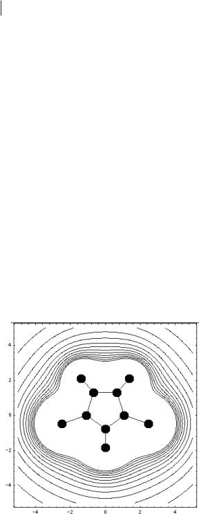
on each molecule, and such models are used for the simulation of systems ranging from simple liquids to biomolecules [1–4]. The short-range interactions are repulsive at short distances, so that the distribution of sites determines the molecular shape in the model. A good description of the electrostatic interactions between different molecules is very important. It is also important to treat the long-range part of the electrostatics carefully. This is best done by the Ewald summation method [6]. Price et al. [7] have developed a model for methyland ethylimidazolium ions with charges on the atomic sites. The charges were taken from a distributed multipole analysis of a good quantum chemical calculation of isolated ions with a reasonablesized basis set with correlations included at the MP2 level. Figure 4.3-1 shows the molecule and the contours of the electrostatic field due to the charges on the sites.

One can see that, while at large distances the contours approach the circular shape expected for an ion, there are considerable distortions near the molecule. The charge is distributed over the ring atoms, the ring protons, and the side chains, particularly on the methyl and methylene groups adjacent to the ring. The charge on the nitrogen atom is negative, while the other charges are all positive. This reflects the electronegativity of the nitrogen atom and is likely to be an important factor in determining the local structure in the liquid. This model was tested by comparison of the predicted and experimental crystal structures.

While this model provides a good description of the electrostatic potential around an isolated ion it does not include the effects of polarization due to the surrounding ions. One might anticipate that a molecule with an aromatic ring would be easily polarizable, and this lack of polarizability is a major shortcoming. The computational cost and problems of parametrizing a polarizable model do not seem worthwhile at this stage of the project. Some justification for this simplification can be taken from recent simulations of triazoles in our group [8]. Triazoles are neutral

Figure 4.3-1: Contours of the electrostatic potential around the dimethylimidazolium ion.

4.3 Molecular Dynamics Simulation Studies 159

molecules with five-membered rings containing nitrogen atoms, which have similarities to the imidazolium ions. Our recent work on simulations of a hybrid model of quantum triazoles dissolved in classical liquid water shows surprisingly small charge fluctuations (amplitude about 0.05 e or less). There is, however, a net polarization of the molecule in aqueous solution compared to in the gas phase. It may be useful in the future to try this type of calculation with imidazolium ions in the ionic liquid, although there are technical problems arising from the fact that the ions are charged. At this stage, simulations are being carried out with the fixed-charge model, which should describe the basic physics of the liquid although, given the comments above, we would not expect quantitative agreement. A further approximation frequently used in simulations of molecular liquids is to replace the methyl and methylene groups by single sites (united atoms). This saves between 35 % and 50 % of the computational effort for dimethylimidazolium salts.

4.3.2

What can we Learn?

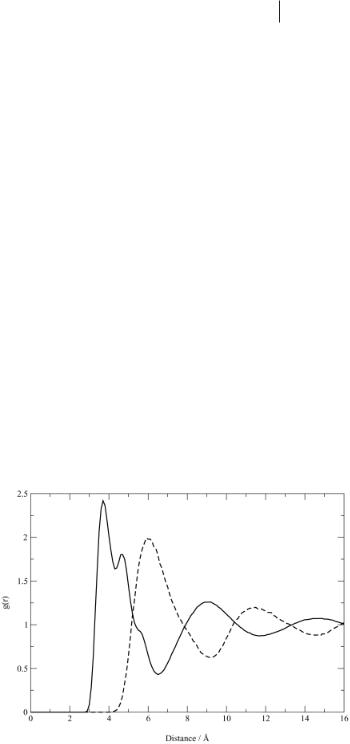
The simulation gives a sequence of configurations: that is, instantaneous positions and velocities of all the atoms in the system. In a molecular dynamics simulation these are a sequence in time, while Monte Carlo simulations give a sequence generated by random moves. These sequences can be analyzed to give structural information, average energies and pressures, and dynamics. Some of this analysis is normally carried out during the simulation (average energies, for example), while other analyses can be carried out later. The problem is to reduce the data to a manageable and comprehensible form. Structural information for liquids is often presented as radial distribution functions gAB(r). These functions show the ratio of the probability density for finding an atom of type A at distance r from an atom of type B relative to the average density of A atoms. Thus, regions where g is greater than unity

Figure 4.3-2: Radial distribution function for dimethylimidazolium and chloride ions relative to chloride. Full line: cation–anion; dashed line: anion–anion.

160 Christof G. Hanke, Ruth M. Lynden-Bell

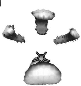
Figure 4.3-3: Three-dimen- sional distribution function of chloride ions relative to dimethylimidazolium ions.

have an enhanced probability of finding atoms of type B, while regions with g less than unity have a reduced probability. Figure 4.3-2 shows g(r) for chloride ions, relative to the center of a dimethylimidazolium ion (or vice versa) and chloride ions relative to a chloride ion. The successive peaks and troughs are out of phase, showing the charge oscillations, which are quite long-ranged.

These are typical of ionic liquids and are familiar in simulations and theories of molten salts. The indications of structure in the first peak show that the local packing is complex. There are 5 to 6 nearest neighbors contributing to this peak. More details can be seen in Figure 4.3-3, which shows a contour surface of the threedimensional probability distribution of chloride ions seen from above the plane of the molecular ion. The shaded regions are places at which there is a high probability of finding the chloride ions relative to any imidazolium ion.

Dynamic information such as reorientational correlation functions and diffusion constants for the ions can readily be obtained. Collective properties such as viscosity can also be calculated in principle, but it is difficult to obtain accurate results in reasonable simulation times. Single-particle properties such as diffusion constants can be determined more easily from simulations. Figure 4.3-4 shows the mean square displacements of cations and anions in dimethylimidazolium chloride at 400 K. The rapid rise at short times is due to rattling of the ions in the cages of neighbors. The amplitude of this motion is about 0.5 Å. After a few picoseconds the mean square displacement in all three directions is a linear function of time and the slope of this portion of the curve gives the diffusion constant. These diffusion constants are about a factor of 10 lower than those in normal molecular liquids at room temperature.

4.3 Molecular Dynamics Simulation Studies 161

Figure 4.3-4: Mean square displacements of cations (full lines) and anions(dashed lines) in x, y, and z directions as a function of time.

Thermodynamic information can also be obtained from simulations. Currently we are measuring the differences in chemical potential of various small molecules in dimethylimidazolium chloride. This involves gradually transforming one molecule into another and is a computationally intensive process. One preliminary result is that the difference in chemical potential of propane and dimethyl ether is about 17.5 kJ/mol. These molecules are similar in size, but differ in their polarity. Not surprisingly, the polar ether is stabilized relative to the non-polar propane in the presence of the ionic liquid. One can also investigate the local arrangement of the ions around the solute and the contribution of different parts of the interaction to the energy. Thus, while both molecules have a favorable Lennard–Jones interaction with the cation, the main electrostatic interaction is that between the chloride ion and the ether molecule.

References

1	J. E. Shea, C. L. Brooks, Annu. Rev.	5	P. A. Madden, M. Wilson, J. Phys.,
	Phys. Chem. 2001, 52, 499.		Condens. Matter 2000, 12, A95.
2	P. La Rocca, P. C. Biggin, D. P. Tiele-	6	M. P. Allen and D. J. Tildesley, Com-
	man, M. S. P. Sansom, Biochim. Bio-		puter Simulation of Liquids, Oxford
	phys. Acta (Biomembranes) 1999, 1462,		University Press, Oxford 1987.
	185.	7	C. G. Hanke, S. L. Price, R. M. Lyn-
3	P. C. Biggin, M. S. P. Sansom,		den-Bell, Mol. Phys. 2001, 99, 801.
	Biophys. Chem. 1999, 76, 161.	8	S. Murdock, G. Sexton, R. M. Lynden-
4	P. A. Bopp, A. Kohlmeyer, E. Spohr,		Bell, in preparation.
	Electrochim. Acta 1998, 43, 2911.

162Joachim Richter, Axel Leuchter, Günter Palmer

4.4

Translational Diffusion

Joachim Richter, Axel Leuchter, and Günter Palmer

4.4.1

Main Aspects and Terms of Translational Diffusion

Looking at translational diffusion in liquid systems, at least two elementary categories have to be taken into consideration: self-diffusion and mutual diffusion [1, 2].

In a liquid that is in thermodynamic equilibrium and which contains only one chemical species,a the particles are in translational motion due to thermal agitation. The term for this motion, which can be characterized as a random walk of the particles, is self-diffusion. It can be quantified by observing the molecular displacements

of the single particles. The self-diffusion coefficient Ds is introduced by the Einstein relationship

	1			r	r	2
Ds	= lim			r (t) − r (0)			(4.4-1)
	t→∞ 6t

where r (t) and r (0) denote the locations of a particle at time t and 0, respectively. The brackets indicate that the ensemble average is used.

However, self-diffusion is not limited to one-component systems. As illustrated in Figure 4.4-1, the random walk of particles of each component in any composition of a multicomponent mixture can be observed.

If a liquid system containing at least two components is not in thermodynamic equilibrium due to concentration inhomogenities, transport of matter occurs. This process is called mutual diffusion. Other synonyms are chemical diffusion, interdiffusion, transport diffusion, and, in the case of systems with two components, binary diffusion.

The description of mass transfer requires a separation of the contributions of convection and mutual diffusion. While convection means macroscopic motion of complete volume elements, mutual diffusion denotes the macroscopically perceptible relative motion of the individual particles due to concentration gradients. Hence, when measuring mutual diffusion coefficients, one has to avoid convection in the system or, at least has to take it into consideration.

Mutual diffusion is usually described by Fick’s first law, written here for a system with two components and one-dimensional diffusion in the z-direction:

−		∂ ci	.	(4.4-2)
Ji	= − Di ∂ z		(i = 1, 2).
a Components are those substances, the				mean any particles in the sense of chemistry
amounts of which can be changed independ-				(atoms, molecules, radicals, ions, electrons)
ently from others, while chemical species				which appear at all in the system [3].

4.4 Translational Diffusion 163

x2 =1:Ds22

x2		0:Ds21	Ds2

D	x1	0:Ds12

Ds1

x1 =1:Ds11

x2

Figure 4.4-1: Self-diffusion and mutual diffusion in a binary mixture. The self-diffusion coefficients are denoted with Ds1 and Ds2, the mutual diffusion coefficient with D. The self-diffusion coefficients of the pure liquids Ds11 and Ds22, respectively, are marked at x1 = 1 and x2 = 1.

Extrapolations x1→0 and x2→0 give the self-diffusion coefficients Ds12 and Ds21.

Equation 4.4-2 describes the flux density Ji (in mol m-2 s-1) of component ι through a reference plane, caused by the concentration gradient ∂ci / ∂z (in mol m-4). The factor Di (in m2 s–1) is called the diffusion coefficient.

Most mutual diffusion experiments use Fick’s second law, which permits the determination of Di from measurements of the concentration distribution as a function of position and time:

	∂c	= D	∂2c
	i		i	(4.4-3)
	∂t		∂z2
		i

Solutions for this second-order differential equation are known for a number of initial and boundary conditions [4].

In a system with two components, one finds experimentally the same values for D1 and D2 because J1 is not independent from J2 . It follows that the system can be described with only one mutual diffusion coefficient D = D1 = D2 .

In the case of systems containing ionic liquids, components and chemical species have to be differentiated. The methanol/[BMIM][PF6] system, for example, consists of two components (methanol and [BMIM][PF6]) but – on the assumption that [BMIM][PF6] is completely dissociated – three chemical species (methanol, [BMIM]+ and [PF6]–). If [BMIM][PF6] is not completely dissociated, one has a fourth species, the undissociated [BMIM][PF6]. From this it follows that the diffusive transport can be described with three and four flux equations, respectively. The fluxes of [BMIM]+

164 Joachim Richter, Axel Leuchter, Günter Palmer

and [PF6]– are not independent, however, because of electroneutrality in each volume of the system. Furthermore, the flux of [BMIM][PF6] is not independent of the flux of the ions because of the dissociation equilibrium. Thus, the number of independent fluxes is reduced to one, and the system can be described with only one mutual diffusion coefficient. In addition, one has four self-diffusion coefficients – Ds(methanol), Ds([BMIM]+), Ds([PF6]–), and Ds([BMIM][PF6]) – so that five diffusion coefficients are necessary to describe the system completely.

4.4.2

Use of Translational Diffusion Coefficients

Following the general trend of looking for a molecular description of the properties of matter, self-diffusion in liquids has become a key quantity for interpretation and modeling of transport in liquids [5]. Self-diffusion coefficients can be combined with other data, such as viscosities, electrical conductivities, densities, etc., in order to evaluate and improve solvodynamic models such as the Stokes–Einstein type [6–9]. From temperature-dependent measurements, activation energies can be calculated by the Arrhenius or the Vogel–Tamman–Fulcher equation (VTF), in order to evaluate models that treat the diffusion process similarly to diffusion in the solid state with jump or hole models [1, 2, 7].

From the molecular point of view, the self-diffusion coefficient is more important than the mutual diffusion coefficient, because the different self-diffusion coefficients give a more detailed description of the single chemical species than the mutual diffusion coefficient, which characterizes the system with only one coefficient. Owing to its cooperative nature, a theoretical description of mutual diffusion is expected to be more complex than one of self-diffusion [5]. Besides that, self-dif- fusion measurements are determinable in pure ionic liquids, while mutual diffusion measurements require mixtures of liquids.

From the applications point of view, mutual diffusion is far more important than self-diffusion, because the transport of matter plays a major role in many physical and chemical processes, such as crystallization, distillation or extraction. Knowledge of mutual diffusion coefficients is hence valuable for modeling and scalingup of these processes.

The need to predict mutual diffusion coefficients from self-diffusion coefficients often arises, and many efforts have been made to understand and predict mutual diffusion data, through approaches such as, for example, the following extension of the Darken equation [5]:

	D = (x2 D21	+ x1D12 ) Γ, with Γ =	d	ln a1	=	d	ln a2	(4.4-4)
			d	ln x1		d	ln x2

where αi is the activity of component i. Γ is denoted as the thermodynamic factor. Systems that are near to ideality can be described satisfactorily with Equation 4.4-4, but the equation does not work very well in systems that are far from thermodynamic ideality, even if the self-diffusion coefficients and activities are known. Since systems with ionic liquids show strong intermolecular forces, there is a need

4.4 Translational Diffusion 165

to find better predictions of the mutual diffusion coefficients from self-diffusion coefficients.

Since the prediction of mutual diffusion coefficients from self-diffusion coefficients is not accurate enough to be used for modeling of chemical processes, complete data sets of mutual and self-diffusion coefficients are necessary and valuable.

4.4.3

Experimental Methods

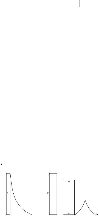
Nowadays, self-diffusion coefficients are almost exclusively measured by NMR methods, through the use of methods such as the 90-δ-180-δ-echo technique (Stejskal and Tanner sequence) [10–12]. The pulse-echo sequence, illustrated in Figure 4.4-2, can be divided into two periods of time τ. After a 90° radio-frequency (RF) pulse the macroscopic magnetization is rotated from the z-axis into the x-y-plane. A gradient pulse of duration δ and magnitude g is applied, so that the spins dephase. After a time τ, a 180° RF pulse reverses the spin precession. A second gradient pulse of equal duration δ and magnitude g follows to tag the spins in the same way. If the spins have not changed their position in the sample, the effects of the two applied gradient pulses compensate each other, and all spins refocus. If the spins have moved due to self-diffusion, the effects of the gradient pulses do not compensate and the echo-amplitude is reduced. The decrease of the amplitude A with the applied gradient is proportional to the movement of the spins and is used to calculate the self-diffusion coefficient.

Popular methods for mutual diffusion measurements in fluid systems are the Taylor dispersion method and interferometric methods, such as Digital Image Holography [13, 14].

With digital image holography it is possible to measure mutual diffusion coefficients in systems that are fairly transparent to laser light and the components of which have a significant difference in their refractive indexes. The main idea of this method is to initiate a diffusion process by creating a so-called step-profile between two mixtures of a binary system with slightly different concentrations. The change

A

90°

180°

δ

δ

τ

g

Figure 4.4-2: Pulse-echo

sequence in an NMR experi-

ment for the measurement of

t=0

t=τ

t=2τ

self-diffusion coefficients.