Ersoy O.K. Diffraction, Fourier optics, and imaging (Wiley, 2006)(ISBN 0471238163)(427s) PEo

68

FRESNEL AND FRAUNHOFER APPROXIMATIONS

where xb and xe are given by

r

D

2

xb ¼

þ x0

lz

2

r

xe ¼

2

D

þ x0

lz 2

Eq. (5.2-15) can be written as

1

xe

1

xb

p 2

p 2

ð5:2-17Þ

Ix ¼ p2

ð ej2v

dv p2

ð ej2v

dv

0

0

The Fresnel integrals C(z) and S(z) are defined by

z

v2

CðzÞ ¼ ð0

cos

p

dv

ð5:2-18Þ

2

z

v2

SðzÞ ¼ ð0

sin

p

dv

ð5:2-19Þ

2

In terms of C(z) and S(z), Eq. (5.2-17) is written as

1

ð5:2-20Þ

Ix ¼ p2 f½CðxeÞ CðxbÞ& þ j½SðxeÞ SðxbÞ&g

The integral above also occurs with respect to y in Eq. (5.2-15). Let it be denoted by Iy, which can be written as

		ye
1		p 2
Iy ¼	p2	ð ej2v dv
	1	yb									ð5:2-21Þ
¼ p2 f½Cðye CðybÞ& þ j½Sðye SðybÞ&g
where			r
									D
		yb ¼	2								þ y0
					lz				2
		r					D
		Ye ¼		2					y0
			lz				2

DIFFRACTION IN THE FRESNEL REGION

69

Equation (5.2-15) for Uðx0; y0; zÞ can now be written as

				ejkz
			Uðx0; y0; zÞ ¼				jxjy	ð5:2-22Þ
					2j
The intensity Iðx0; y0; zÞ ¼ jUðx0; y0; zÞj2 can be written as
Iðx0; y0; zÞ ¼	1		f½CðxeÞ CðxbÞ&2 þ ½SðxeÞ SðxbÞ&2g
		4
	f½CðyeÞ CðybÞ&2 þ ½SðyeÞ SðybÞ&2g							ð5:2-23Þ
The Fresnel number NF is defined by
			NF ¼	D2				ð5:2-24Þ
				4lz

For constant D and l, NF decreases as z increases.

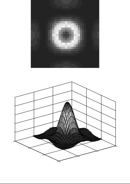
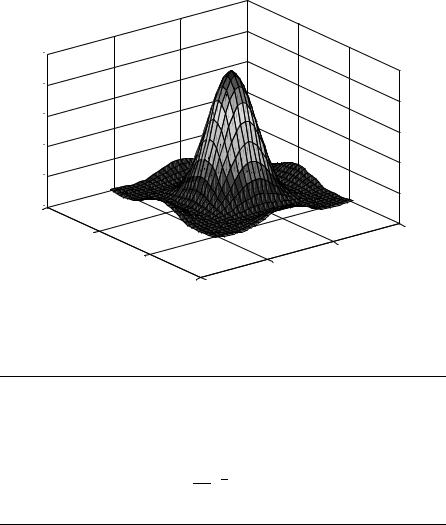
The Fresnel diffraction intensity from a square aperture is visualized in Figures 5.2–5.5. As z gets less, the intensity starts resembling the shape of the input square aperture. This is further justified in Example 5.5. Figure 5.2 shows the image of the square aperture used. Figure 5.3 is the Fresnel intensity diffraction pattern from the square aperture. Figure 5.4 is the same intensity diffraction pattern as a 3-D plot.

Figure 5.2. The input square aperture for diffraction studies.

70	FRESNEL AND FRAUNHOFER APPROXIMATIONS

Figure 5.3. The intensity diffraction pattern from a square aperture in the Fresnel region.

100

80

60

40

20

0

0.5

0	0.5
	0

–0.5

–0.5

–1 –1

Figure 5.4. The same intensity diffraction pattern from the square aperture in the Fresnel region as a 3-D plot.

EXAMPLE 5.5 Using the Fresnel approximation, show that the intensity of the diffracted beam from a rectangular aperture looks like the rectangular aperture for small z.

Solution: The intensity pattern from the rectangular aperture is given by Eq. (5.2-22) where Dx and Dy are used instead of D along the x- and y-directions, respectively.

DIFFRACTION IN THE FRESNEL REGION

71

The variables for very small z can be written as

r

1

2

D

! (

x0 > Dx=2

xb ¼

lz

2

þ x0

1x0 < Dx=2

r

1

< Dx=2

2 D

x0

xe ¼

lz 2

x0

! ( 1 x0 > Dx=2

r

1

2 D

! (

1 y0 > Dy=2

yb ¼

lz

2

þ y0

y0 < Dy=2

r

1

< Dy=2

2

D

y0

ye ¼

lz

2

y0

! ( 1 y0 > Dy=2

The asymptotic limits of cosine and sine integrals are given by

Cð1Þ ¼ Sð1Þ ¼ 0:5; Cð 1Þ ¼ Sð 1Þ ¼ 0:5

Consequently, Eq. (5.2-22) becomes

x0

rect

y0

Iðx0; y0; zÞ ’ rect

D

D

for small z.

EXAMPLE 5.6 Show under what conditions the angular spectrum method reduces to the Fresnel approximation.

Solution: The transfer function in the angular spectrum method is given by

			(	p	q
HA	ð	fx; fy	Þ ¼	ejz k2 4p2ðfx2þfy2Þ	fx2 þ fy2 < l1
				0	otherwise

The transfer function in the Fresnel approximation is given by

HFðfx; fyÞ ¼ ejkze jplzðfx2þfy2Þ

If

q						4p2ð fx2 þ fy2Þ
	2	2	2	2
k		4p	ð fx	þ fy	Þ k	2k

that corresponds to keeping the first two terms of the Taylor expansion HAð fx; fyÞ equals HFð fx; fyÞ. The approximation above is valid when jlfxj, jlfyj 1. In conclusion, the Fresnel approximation and the angular spectrum method are approximately equivalent for small angles of diffraction.

72	FRESNEL AND FRAUNHOFER APPROXIMATIONS

5.3FFT IMPLEMENTATION OF FRESNEL DIFFRACTION

Fresnel diffraction can be implemented either as convolution given by Eq. (5.2-10) or by directly using the DFT after discretizing Eq. (5.2-13). The convolution implementation is similar to the implementation of the method of the angular spectrum of plane waves. The second approach is discussed below.

Let Uðm1; m2; 0Þ ¼ Uð xm1; ym2; 0Þ be the discretized u(x,y,0). Thus, x and y are discretized as xm1 and xm2, respectively. Similarly, x0 and y0 are discretized as x0n1 and x0n2, respectively. We write

U0ðm1; m2; 0Þ ¼ Uðm1; m2; 0Þej	k	½ð xm1Þ2þð ym2Þ2&	ð5:3-1Þ
	2z

In order to use the FFT, the Fourier kernel in Eq. (5.2-13) must be expressed as

e j2lpzðx0xþy0yÞ ¼ e j2lpzð x x0n1m1þ y y0n2m2Þ ¼ e j2p

n m

1

n m

2

1

þ

2

ð5:3-2Þ

N1

N2

where N1 N2 is the size of the FFT to be used. Hence,

2p

2p

n1m1

x0x ¼

x x0n1m1 ¼ 2p

lz

lz

N1

This yields

x x0 ¼

lz

ð5:3-3Þ

N1

Similarly, we have

y y0 ¼

lz

ð5:3-4Þ

N2

In other words, small x or y gives large x0 or y0 and vice versa, respectively. Equations (5.3-3) and (5.3-4) can be compared to Eq. (4.4-12) for the angular spectrum method. For fx ¼ x0=lz and fy ¼ y0=lz, these equations are the same. However, now the output is directly given by Eq. (5.2-3), there is no inverse transform to be computed, and hence the input and output windows can be of different sizes.

	ð			Þ		2	2
In order to use the FFT, U0		m1	; m2; 0		is shifted by	N1	;	N2	, as discussed
previously in Section 4.4. Suppose the result is U00ðm1; m2; 0Þ.

The discretized output wave Uðn1; n2; zÞ ¼ Uð x0n1; y0n2; zÞ is expressed as

ejkz

k

2

2

X X

n1m1

n2m2

N1

1

N2

1

Uðn1; n2; zÞ ¼

jlz

ej

2z

½ð x0n1

Þ

þð y0n2Þ

& x y m1

¼

0

m2

¼

0 U00ðm1; m2; 0Þe j2p

N1

þ

N2

ð5:3-5Þ

Uðn1; n2; zÞ is shifted again by

N1

;

N2

in order to correspond to the real wave.

2

2

PARAXIAL WAVE EQUATION

73

EXAMPLE 5.7 Consider Example 4.4. With the same definitions used in that example, the pseudo program for Fresnel diffraction can be written as

u1 ¼ u exp j k ðx2 þ y2Þ

2z u1p ¼fftshiftðu1Þ

ejkz

u3 ¼ jlz ej2kzðx20þy20Þ u2

U¼fftshiftðu3Þ

5.4PARAXIAL WAVE EQUATION

The Fresnel approximation is actually a solution of the paraxial wave equation derived below. Consider the Helmholtz equation . If the field is assumed to be propagating mainly along the z-direction, it can be expressed as

Uðx; y; zÞ ¼ U0ðx; y; zÞejkz

ð5:4-1Þ

where U0ðx; y; zÞ is assumed to be a slowly varying function of z. Substituting Eq. (5.4-1) in the Helmholtz equation yields

r2U0	d	ð5:4-2Þ
	þ 2jk dz U0 ¼ 0

As U0ðx; y; zÞ is a slowly varying function of z, Eq. (5.4-2) can be approximated as

d2U0 þ d2U0 þ 2jk d U0 ¼ 0 dx2 dy2 dz

Equation (5.4-3) is called the paraxial wave equation. Consider

1 jkðx2þy2Þ

U1ðx; yÞ ¼ jlz e 2z

ð5:4-3Þ

ð5:4-4Þ

It is easy to show that U1 is a solution of Eq. (5.4-3). As Eq. (5.4-3) is linear and shift invariant, U1ðx x1; y y1Þ for arbitrary x1 and y1 is also a solution. Superimposing

74 FRESNEL AND FRAUNHOFER APPROXIMATIONS

such solutions, a general solution is found as

Uðx; y; zÞ ¼ jlz ðð gðx1; y1Þe

ðð

Þ

2z

Þ2

dx1dy1

ð5:4-5Þ

1

jk

x

x1

2þðy y1

Þ

Consider the Fresnel approximation given by

Uðx0; y0; zÞ ¼ jlz ðð Uðx; y; 0Þe

ðð

Þ

2z

dxdy

ð5:4-6Þ

1

jk

x0

x

2þðy0 yÞ2

Þ

Choosing gðx; yÞ ¼ Uðx; y; 0Þ, it is observed that Eqs. (5.4-5) and (5.4-6) are the same. Hence, the Fresnel approximation is a solution of the paraxial wave equation.

5.5DIFFRACTION IN THE FRAUNHOFER REGION

Consider Eq. (5.2-14). If
		k	ðx2 þ y2Þmax		kL2
z				¼		1	;	ð5:5-1Þ
	2					2

then, U0ðx; y; 0Þ is approximately equal to U(x,y,0). When this happens, the Fraunhofer region is valid, and Eq. (5.2-13) becomes

Uðx0; y0	; zÞ ¼ jlz ej2zðx0					þy0Þ	ðð	Uðx; y; 0Þe jlzðx0xþy0yÞdxdy			ð5:5-2Þ
	ejkz			k 2		2	1		2p
							1

Aside from multiplicative amplitude and phase factors, Uðx0; y0; zÞ is observed to be the 2-D Fourier transform of U(x,y,0) at frequencies fx ¼ x0=lz and fy ¼ y0=lz. It is also observed that diffraction in the Fraunhofer region does not have the form of a convolution.

EXAMPLE 5.8 Find the wave field in the Fraunhofer region due to a wave emanating from a circular aperture of diameter D at z ¼ 0.

Solution: The circular aperture of diameter D means

Uðx; y; 0Þ ¼ cylðr=DÞ

p where r ¼ x2 þ y2.

From Example 2.6, the 2-D Fourier transform of U(x,y,0) is given by

	D2p		q
Uðx; y; 0Þ $	4		somb D fx2 þ fy2

DIFFRACTION IN THE FRAUNHOFER REGION

75

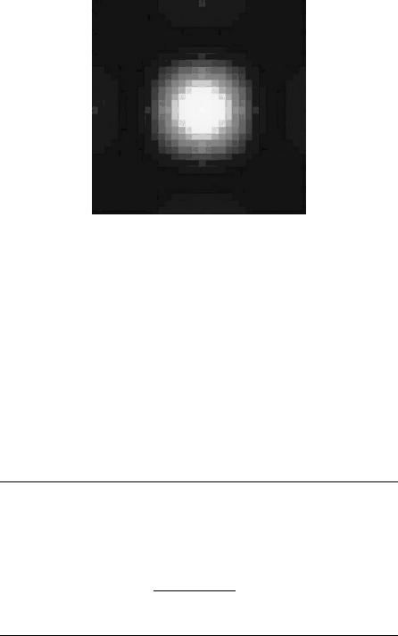
Figure 5.5. The intensity diffraction pattern from a square aperture in the Fraunhofer region.

where fx ¼ x0=lz and fy ¼ y0=lz. Using Eq. (5.5-2) gives

ð

Þ ¼

l

2

q

2

e

jkz

2

k 2

D p

U x0; y0; z

j

z

ej

2z

ðx0

þy0

Þ

4

somb D

fx2 þ fy2

The intensity distribution equal to U2ðx0; y0; zÞ is known as the Airy pattern. It is

	given by				h	q i
	Iðx0; y0; zÞ ¼	kD2		2			2
					somb	D fx2 þ fy2
		8z

The Fraunhofer diffraction intensity from the same square aperture of Figures 5.2 is visualized in Figures 5.5 and 5.6. Figure 5.5 is the Fraunhofer intensity diffraction pattern from the square aperture. Figure 5.6 is the same intensity diffraction pattern as a 3-D plot.

EXAMPLE 5.9 Determine when the Fraunhofer region is valid if the wavelength is 0.6 m (red light) and an aperture width of 2.5 cm is used.

Solution:

z			kL12				pL12
					¼
			2				l
	pL12		¼	p ð1:25 10 2Þ2					¼	830 m
	l
						0:6 10 6

This large distance will be much reduced when the lenses are discussed in Chapter 8.

76	FRESNEL AND FRAUNHOFER APPROXIMATIONS

100

80

60

40

20

0

0.5

	0	0.5
		0

–0.5

–0.5

–1 –1

Figure 5.6. The same intensity diffraction pattern from the square aperture in the Fraunhofer region as a 3-D plot.

EXAMPLE 5.10 Consider Example 5.7. With the same definitions used in that example, the pseudo program for Fresnel diffraction can be written as

u1 ¼ fftshiftðu1Þ u2 ¼ fftðu1Þ

ejkz

u3 ¼ jlz ej2kzðx20þy20Þ u2

U¼ fftshiftðu3Þ

5.6DIFFRACTION GRATINGS

Diffraction gratings are often analyzed and synthesized by using Fresnel and Fraunhofer approximations. Some major application areas for diffraction gratings are spectroscopy, spectroscopic imaging, optical communications, and networking.

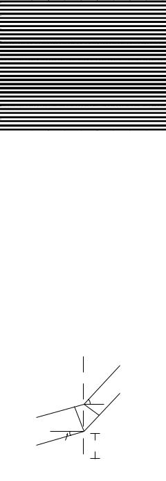
A diffraction grating is an optical device that periodically modulates the amplitude or the phase of an incident wave. Both the amplitude and the phase may also be modulated. An array of alternating opaque and transparent regions is called a transmission amplitude grating. Such a grating is shown in Figures 5.7 and 5.8.

DIFFRACTION GRATINGS

77

Figure 5.7. Planar view of a transmission amplitude grating.

If the entire grating is transparent, but varies periodically in optical thickness, it is called a transmission phase grating. A reflective material with periodic surface relief also produces distinct phase relationships upon reflection of a wave. These are known as reflection phase gratings. Reflecting diffraction gratings can also be generated by fabricating periodically ruled thin films of aluminum evaporated on a glass substrate.

Diffraction gratings are very effective to separate a wave into different wavelengths with high resolution. In the simplest case, a grating can be considered as a large number of parallel, closely spaced slits. Regardless of the number of slits, the peak intensity occurs at diffraction angles governed by the following grating equation:

d sin fm ¼ ml

ð5:6-1Þ

where d is the spacing between the slits, m is an integer called diffraction order, and f is the diffraction angle. Equation (5.6-1) shows that waves at different

mth order

qm

qi d

Figure 5.8. Periodic amplitude grating.