Ersoy O.K. Diffraction, Fourier optics, and imaging (Wiley, 2006)(ISBN 0471238163)(427s) PEo

48 SCALAR DIFFRACTION THEORY

where x, y, fx, fy are the sampling intervals, and n1, m1, as well as n2, m2 are integers satisfying

M1n1; m1 M1	4		4-2	Þ
M2n2; m2 M2	ð	:
We will write Uð xn1; yn2; zÞ and Að fxm1; fym2; zÞ as	U½n1; n2; z&		and

A½m1; m2; z&, respectively. In terms of discretized space and frequency variables, Eqs. (4.3-2) and (4.3-8) are approximated by

	X1		X2	U½n1		; 0&e j2pð fx xn1m1þ fy yn2m2Þ			ð4:4-3Þ
A½m1; m2; 0& ¼ x y		n	n		; n2
½ 1 2 & ¼	x y	m1	m2	½	1	2 &	ð Þ
	f f	X X					jzpk2 4p2 fx2m2	fy2m2
U n ; n ; z				A m ; m ; 0 e			1þ	2
	e j2pð fx xn1m1þ fy yn2m2Þ								ð4:4-4Þ

M1 and M2 should be chosen such that the inequality (4.3-13) is satisfied if evanescent waves are to be neglected. An approximation is to choose a rectangular region in the Fourier domain such that

jkxj ¼ 2pj fxj k						ð4:4-5Þ
jkyj ¼ 2pj fyj k						ð4:4-6Þ
Then, the following must be satisfied:
1						ð4:4-7Þ
j fx max j ¼ j fy max j ¼
					l
Choosing M ¼ M1 ¼ M2, f ¼ fx ¼ fy gives
1						ð4:4-8Þ
fmax ¼ fM ¼
			l
Hence,
1
M ¼						ð4:4-9Þ
	f l

In practice, it is often true that fx max and fy max Eq. (4.4-8) becomes

M ¼ fx max

1

fx

are less than 1=l. If they are known,

ð4:4-10Þ

FFT IMPLEMENTATION OF THE ANGULAR SPECTRUM OF PLANE WAVES

49

in the x-direction, and

M2 ¼	fy max	ð4:4-11Þ
	fy

in the y-direction. Assuming fx max ¼ fy max , fx ¼ fy ¼ f gives M ¼ Mx ¼ My. FFTs of length N will be assumed to be used along the two directions so that

¼ x ¼ y, and f ¼ fx ¼ fy. How N is related to M is discussed below. In order to be able to use the FFT, the following must be valid:

f ¼	1	ð4:4-12Þ
	N

U½n1; n2; z& and A½m1; m2; z& for any z are also assumed to be periodic with period N. Hence, for m1, m2, n1, n20, they satisfy

U½ n1; n2; z& ¼ U½N n1; n2; z&
U½n1;	n2; z& ¼ U½n1; N n2; z&
U½ n1;	n2; z& ¼ U½N n1; N n2	; z&
A½ m1; m2; z& ¼ A½N m1; m2; z&		ð4:4-13Þ
A½m1;	m2; z& ¼ A½m1; N m2; z&
A½ m1;	m2; z& ¼ A½N m1; N m2; z&

Mapping of negative indices to positive indices is shown in Figure 4.2. Using Eq. (4.4-13), Eqs. (4.4-3) and (4.4-4) can be written as follows:

X X
N 1 N	1	2p
A½m1; m2; 0& ¼ 2	U½n1; n2; 0&e j	N	ðn1m1þn2m2Þ			ð4:4-14Þ
n1¼ 0 n2¼ 0
X X
N 1	N 1
U½n1; n2; z& ¼ ð f 0Þ2	A½m1; m2; z&e j			2p	ðm1n1þm2n2Þ	ð4:4-15Þ
				N

m1¼ 0 m2¼ 0

y

IV

III

II

I

II

III

IV

x

Figure 4.2. Mapping of negative index regions to positive index regions to use the FFT.

50

SCALAR DIFFRACTION THEORY

where

pð Þ ð

½

1;

2; & ¼

½ 1;

2;

&

ð :

Þ

A

m

m z

A m

m

0

e jz

k2 4p2 fx 2 m12þm22Þ

4

4-16

where m1 and m2 satisfy condition (4.4-2). A½m1; m2; z& is also assumed to be periodic with period N:

A½	m1; m2; z& ¼ A½N m1; m2; z&		ð4:4-17Þ
A½m1;		m2; z& ¼ A½m1; N m2; z&
A½	m1;	m2; z& ¼ A½N m1; N m2; z&

Note that the periodicity condition due to the use of the FFT causes aliasing because circular convolution rather than linear convolution is computed. In order to reduce aliasing, the input and output apertures can be zero padded to a size, say,

M0 ¼ 2M. Then, N can be chosen as follows:					ð4:4-18Þ
N ¼		2M00	þ 1	N odd
		2M		N even

In addition, FFT algorithms are usually more efficient when N is a power of 2. Hence, N may actually be chosen larger than the value computed above to make it a power of 2.

Equations (4.4-15) and (4.4-16) can now be written as

¼	¼	p
X X
N 1	N 1	A½m1; m2; 0&e jz k2 4p2ð fxÞ2ðm12þm22Þ e j	2p
U½n1; n2; z& ¼ ð f Þ2 m1 0 m2 0			N	ðn1m1þn2m2Þ

ð4:4-19Þ

Equation (4.4-19) is in the form of an inverse 2-D DFT except for a normalization factor.

As ð f Þ2 ¼ N12, 2 and ð f Þ2 in Eqs. (4.4-14) and (4.4-15) can be omitted, and only one of these equations, say, Eq. (4.4-14) is multiplied by N12.

In summary, the procedure to obtain Uðx; y; zÞ from Uðx; y; 0Þ with the angular spectrum method and the FFT is as follows:

1.Generate U½n1; n2; 0& as discussed above.

2.Compute A½m1; m2; 0& by FFT according to Eq. (4.4-14).

3.Compute A½m1; m2; z& according to Eq. (4.4-16).

4.Compute U½n1; n2; z& by FFT according to Eq. (4.4-19).

5.Arrange U½n1; n2; z& according to Eq. (4.4-13) so that negative space coordinates are regenerated.

The results discussed above can be easily generalized to different number of data points along the x- and y-directions.

FFT IMPLEMENTATION OF THE ANGULAR SPECTRUM OF PLANE WAVES

51

EXAMPLE 4.4 Suppose that the following definitions are made: fftshift: operations defined by Eqs. (4.4.13) and (4.417)

fft2, ifft2: routines for 2-D FFT and inverse FFT, respectively H: transfer function given by Eq. (4.3.14)

u, U: input and output fields, respectively Using these, an ASM program can be written as u1¼fftshift ((fft2(fftshift(u))))

u2¼H u1 U¼fftshift(ifft2(fftshift(u2)))

Show that this program can be reduced to u1¼fftshift((fft2(u)))

u2¼H u1 U¼ifft2(fftshift(u2))

Solution: The difference between the two programs is reduction of fftshift in the first and third steps of the program. This is possible because of the following property of

the DFT shown in 1-D:

½

& ¼

½

&

If u0

½

n

& ¼

u n

2

k

e

jpk. When the fftshift in the first step of the

N , then U0

U

k

skipped, the end result is the phase shift e

jpk

. When the fftshift in the third

program is

step is skipped, the same phase shift causes the output U to be correctly generated.

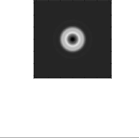
EXAMPLE 4.5 Suppose the parameters are given as follows:

Input size: 32 32	N ¼ 512
l ¼ 0:0005	z ¼ 1000

The units above can be in mm. A Gaussian input field is given by

Uðx; y; 0Þ ¼ exp½ 0:01pðx2 þ y2Þ&

The input field intensity is shown in Figure 4.3. The corresponding output field intensity computed with the ASM is shown in Figure 4.4. If z is changed to 100, the corresponding output field is as shown in Figure 4.5. Thus, the ASM can be used for any distance z. As expected, if the input field is Gaussian, the output field also remains Gaussian.

EXAMPLE 4.6 Determine the impulse response function corresponding to the transfer function given by Eq. (4.3.14).

Solution: The impulse response is the inverse Fourier transform of the transfer function:

	1	1
hðx; yÞ ¼	ð	ð	e jkz½1 l2fx2 l2fy2&1=2e j2pð fxxþfyyÞdfxdfy	ð4:4-20Þ

11

52	SCALAR DIFFRACTION THEORY

–15

–10

–5

0

5

10

15

–15

–10

–5

0

5

10

15

Figure 4.3. The input Gaussian field intensity.

where ax2 þ ay2 ¼ l2ð fx2 þ fy2Þ is used. We note				that	Hð fx; fyÞ has cylindrical
symmetry. For this reason, it is better to use cylindrical coordinates by letting
x ¼ r cos y; y ¼ r sin y; fx ¼ cos ;				and	fy ¼ sin
In cylindrical coordinates, Eq. (4.4-20) becomes [Stark, 1982]:
1
hðrÞ ¼	1	ð0	e zðt2 k2Þ1=2 J0ð2pr Þ d
	2p

–15

–10

–5

0

5

10

15

–15

–10

–5

0

5

10

15

Figure 4.4. The output field intensity when z ¼ 1000.

THE KIRCHOFF THEORY OF DIFFRACTION

53

–15

–10

–5

0

5

10

15

–15

–10

–5

0

5

10

15

Figure 4.5. The output field intensity when z ¼ 100.

where J0ð Þ is the Bessel function of the first kind of zeroth order. The integral above can be further evaluated as

jk z2

r2 1=2

"1 þ

#

hðrÞ ¼

e ½

þ &

z

1

ð4:4-21Þ

jl z2

r2

&

1=2

½

z2

r2

&

1=2

jk z2

r2

&

1=2

½ þ

þ

½

þ

EXAMPLE 4.7 Determine the wave field due to a point source modeled by

Uðx; y; 0Þ ¼ dðx 3Þdðy 4Þ:

Solution: The output wave field is given by

Uðx; y; zÞ ¼ Uðx; y; 0Þ hðx; y; zÞ

1

2

2

2

1=2

’ dðx

3Þdðy

4Þ

e jk½z

þx

þy

&

jlz

1

2

2

2

1=2

’

e jk½z

þðx 3Þ þðy 4Þ

&

jlz

4.5THE KIRCHOFF THEORY OF DIFFRACTION

The propagation of the angular spectrum of plane waves as discussed in Section 4.5 does characterize diffraction. However, diffraction can also be treated by starting

54 SCALAR DIFFRACTION THEORY

n

V S

Figure 4.6. The volume and its surface used in Green’s theorem.

with the Helmholtz equation and converting it to an integral equation using Green’s theorem.

Green’s theorem involves two complex-valued functions UðrÞ and GðrÞ (Green’s function). We let S be a closed surface surrounding a volume V, as shown in Figure 4.6.

If U and G, their first and second partial derivatives respectively, are singlevalued and continuous, without any singular points within and on S, Green’s theorem states that

ð Vð ððGr2U Ur2GÞdv ¼	ððS	G @n		U @n ds		ð4:5-1Þ
			@U		@G

where @=@n indicates a partial derivative in the outward normal direction at each point of S. In our case, U corresponds to the wave field.

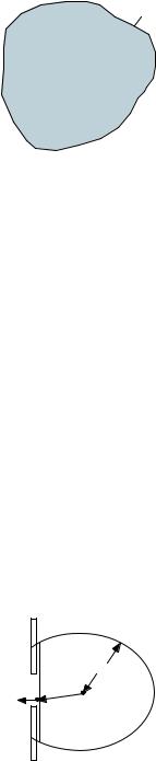
Consider the propagation of an arbitrary wave field incident on a screen at an initial plane at z ¼ 0 to the observation plane at some z. The geometry to be used is shown in Figure 4.7. In this figure, P0 is a point in the observation plane, and P1, which can be an arbitrary point in space, is shown as a point at the initial plane. The closed surface is the sum of the surfaces S0 and S1. There are two choices of the Green’s function that lead us to a useful integral representation of diffraction. They are discussed below.

S0

S1

R

A	r01
n	P0
	P1

Figure 4.7. The geometry used in Kirchoff formulation of diffraction.

THE KIRCHOFF THEORY OF DIFFRACTION

55

4.5.1Kirchoff Theory of Diffraction

The Green function chosen by Kirchhoff is a spherical wave given by

GðrÞ ¼	e jkr01	ð4:5-2Þ
	r01

where r is the position vector pointing from P0 to P1, and r01is the corresponding distance, given by

r01 ¼ ½ðx0 xÞ2 þ ðy0 yÞ2 þ z2&1=2

ð4:5-3Þ

UðrÞ satisfies the Helmholtz equation. As GðrÞ is an expanding spherical wave, it also satisfies the Helmholtz equation:

r2GðrÞ þ k2GðrÞ ¼ 0

ð4:5-4Þ

The left hand side of Eq. (4.5-1) can now be written as

ð Vð ð½Gr2U Ur2G&dV ¼ ð Vð ð k2½UG UG&dv ¼ 0

Hence, Eq. (4.5-1) becomes

@n ds ¼ 0

ððS G @n

U

ð4:5-5Þ

@U

@G

On the surface S0 of Figure 4.7, we have

GðrÞ ¼

e jkR

R

R

R

@n

@n ¼

@GðrÞ

jk

1

e jkR

@U

jkU

The part of the last integral in Eq. (4.5-1) over S0 becomes

@U

IS2 ¼ ð GðrÞ

jkU ds

@n

S0

@U

¼ ð GðrÞ

jkU R2dw

@n

¼ ð e jkR R @n

jkU dw

@U

56	SCALAR DIFFRACTION THEORY

where is the solid angle subtended by S0 at P0. The last integral goes to zero as

R ! 1 if

Rlim R	@U	jkU ¼ 0	ð4:5-6Þ
	@n
!1

This condition is known as the Sommerfeld radiation condition and leads us to results in agreement with experiments.

What remains is the integral over S1, which is an infinite opaque plane except for the open aperture to be denoted by A. Two commonly used approximations to the boundary conditions for diffraction by apertures in plane screens are the Debye approximation and the Kirchhoff approximation [Goodman, 2004]. In the Debye approximation, the angular spectrum of the incident field has an abrupt cutoff such that only those plane waves traveling in certain directions passed the aperture are maintained. For example, the direction of travel from the aperture may be toward a focal point. Then, the field in the focal region is a superposition of plane waves whose propagation directions are inside the geometrical cone whose apex is the focal point and whose base is the aperture.

The Kirchhoff approximation is more commonly used. If an aperture A is on plane z ¼ 0, as shown in Figure 4.7, the Kirchhoff approximation on the plane z ¼ 0þ is given by the following equations:

Uðx; y; 0þÞ ¼ ( Uðx;0y; 0Þ	inside A	ð4:5-7Þ
	outside A

@ U		Þ z¼0þ		8	@		Uðx; y; zÞ z¼0 :
	x; y; z		¼			@z
@z ð				>	0
				<

	>
	:

inside A

ð4:5-8Þ

outside A

It is observed that Uðx; y; zÞ and its partial derivative in the z-direction are discontinuous outside the aperture and continuous inside the aperture at z ¼ 0 according to the Kirchhoff approximation. These conditions are also called Kirchoff boundary conditions. They lead us to the following solution for UðP0Þ:

UðP0	Þ ¼ 4p ððA G		@n	U @n ds		ð4:5-9Þ
	1		@U		@G

4.5.2Fresnel–Kirchoff Diffraction Formula

Assuming r01 is many optical wavelengths, the following approximation can be made:

@	G P			@			e jkr01	¼ cosðyÞ jk	1	GðP1
	ð	1Þ	¼								Þ jk cosðyÞGðP1Þ ð4:5-10Þ
	@n			@n			r01		r01

THE RAYLEIGH–SOMMERFELD THEORY OF DIFFRACTION

57

P2	r01	P0
	A

n

P1

Figure 4.8. Spherical wave illumination of a plane aperture.

Hence, Eq. (4.5-9) becomes

UðP0	Þ ¼ 4p ððA		r01	@n	jk cosðyÞU ds
	1		e jkr01	@U

Let us apply this equation to the case of UðP1Þ being a spherical wave originating at a point P2 as shown in Figure 4.8. Denoting the distance between P1 and P2 as r21, and the angle between n and r21 by y2, we have

UðP1Þ ¼

Gðr21Þ

e jkr21

r21

@UðP1

Þ

jk cos

ðy2

Þ

G r

Þ

@n

ð 21

Hence, we get

ððA

rð21r01

Þ ds

UðP0

Þ ¼ jl

ðyÞ

2

ðy

ð4:5-11Þ

1

e jk r21

þr01Þ

cos

cos

2

This result is known as the Fresnel–Kirchoff diffraction formula, valid for diffraction of a spherical wave by a plane aperture.

4.6THE RAYLEIGH–SOMMERFELD THEORY OF DIFFRACTION

The use of the Green’s function given by Eq. (4.5-2) together with a number of simplifying assumptions leads us to the Fresnel–Kirchhoff diffraction formula as discussed above. However, there are certain inconsistencies in this formulation. These inconsistencies were later removed by Sommerfeld by using the following