Modulation and Demodulation of Biomedical Signals						461
				CLOCK
		+ 5 V
vm				CP Q
			vc
		COMP.	(TTL)	D	_	Vo
	vr’
					Q
				DFF		(TTL)
						+1 V
			(LPF)		(Absval.)
		−2.4 V		vf
			C
					R	−2.4 V
		vr
			OA
			(Int.)			(AM)
	−Vbias			A

C

(AM)

R

^

vm

−2.4 V
(LPF)	(Absval.)
Vo	vf
(TTL)

B	+1 V

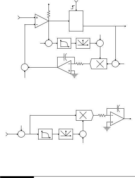
FIGURE 11.18

(A) Circuit for an adaptive delta modulator. (B) Demodulator for ADM. A long time-constant LPF is generally used instead of an ideal integrator for filtering vm.

11.7 Chapter Summary

Broadly speaking, modulation is a process in which a low-frequency modulating signal acts on a high-frequency carrier wave in some way so that the high-frequency modulated carrier can be transmitted (e.g., as radio waves, ultrasound waves, light waves, etc.) to a suitable receiver; after this the process of demodulation occurs, recovering the modulating signal. In the

© 2004 by CRC Press LLC

462	Analysis and Application of Analog Electronic Circuits

frequency domain, the low-frequency power spectrum of the signal is translated upward in frequency to lie around the carrier frequency. A major purpose of modulation is to permit long-range transmission of the modulating signal by a relatively noise-free modality.

Why transmit modulated carriers? After all, traditional short-distance telephony transmits audio information directly on telephone lines. The answer lies in the signal spectrum. The low frequencies associated with many endogenous physiological signals cannot be transmitted by conventional voice telephony; modulation must be used. The carrier modality can be radio waves, ultrasound, or light on fiber optic cables. For example, when the modulating signal is an ECG, its power spectrum is too low for direct transmission by telephone lines. However, the ECG can narrow-band fre- quency-modulate (NBFM) an audio-frequency carrier that can be transmitted on phone lines and demodulated at the receiver. In a case in which an ambulance is en route carrying a patient, the ECG can directly NBFM an RF carrier, which is received and demodulated at the hospital’s ER.

Subcarrier modulation can be used as well. Here several low-frequency physiological signals such as ECG, blood pressure, and respiration can NBFM an audio subcarrier, each with a different frequency. The modulated subcarriers are added together and used to modulate amplitude of frequency of an RF carrier, which is transmitted. Subcarrier FM can also be used with ultrasonic “tags” to monitor marine animals such as whales and dolphins. The tag is attached to the animal and reports such parameters as depth, water temperature, heart rate, etc. The subcarriers are separated following detection at the receiver by band-pass filters and then demodulated.

The section about AM examined the process in the frequency domain and gave examples of selected circuits used in AM and single-sideband AM. Double-sideband, suppressed-carrier AM was shown to be the simple result of multiplying the carrier by the modulating signal. Examples of DSBSCM were shown to include Wheatstone bridge outputs given ac carrier excitation and the output of an LVDT. Broadband and narrowband FM were examined theoretically; circuits and systems used to generate NBFM, such as the phaselocked loop (PLL), were described as well. Integraland relaxation-pulse frequency modulation were introduced.

The section on demodulation illustrated circuits and systems used to demodulate AM, DSBSCM, FM, and NBFM signals. Again, the PLL was shown to be effective at demodulation. Modulation of digital (e.g., TTL, ECL) carriers includes FM and – (sigma–delta) modulation, pulse-width or duty-cycle modulation, and adaptive delta modulation. Means of demodulating digital modulated signals were described.

Home Problems

11.1An analog pulse instantaneous pulse frequency demodulator (IPFD) must generate a hyperbolic (not exponential) capacitor discharge waveform in order to convert interpulse intervals to elements of instantaneous frequency

© 2004 by CRC Press LLC

Modulation and Demodulation of Biomedical Signals				463
		R/10	R
		R
		vc	IOA	v3
	inl	vc2 /10	−vc
C		AM
		R	R

vc R

IOA

IOA

vc(t) to S&H

vc(t)

10 V

vc(t) =

100

t + 0.001

tk	tk + 1 ms	tk+1	t

0

(local time origin)

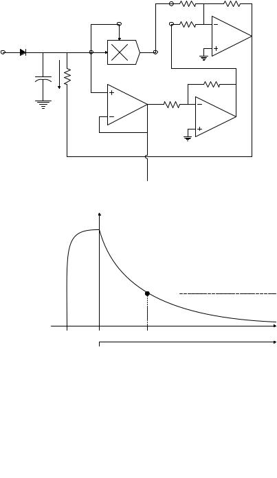
FIGURE P11.1

(IF). IF is defined as the reciprocal of the interval between two adjacent impulses in a sequence of pulses. When the (k + 1)th pulse in a sequence occurs, the kth hyperbolic waveform voltage is sampled and held, generating the kth element of IF, which is held until the (k + 2)th pulse occurs, etc. The capacitor discharge will be a portion of a hyperbola for t ≥ 1 MS following the occurrence of each pulse. Mathematically, this can be stated:

	v (t) =	C β
		t + τo
	c

© 2004 by CRC Press LLC

464	Analysis and Application of Analog Electronic Circuits

where Vcmax = 10 V; C = 1 μF; and τo = C/(βVcmax) = 0.001 sec. It can be shown that if the capacitor is allowed to discharge into a nonlinear conductance so that: inl (t) = β vc(t)2, the preceding hyperbolic vc(t) will occur (Northrop, 1997). Time t is measured from (tk + 0.001) sec (see the timing diagram below the schematic). This means that if tk+1 = (tk + 0.001), vc(0) = 10 V for an IF of 1000 pps. Note that prior to each discharge cycle, C is charged through the diode to +10 V.

In this problem, you are to analyze and design the active circuit of Figure P11.1 that causes inl (t) = βvc(t)2 and generates the hyperbolic vc(t) described. That is, find the numerical value of R required, given the preceding parameter values. Also find the numerical values for β and the peak inl (t).

11.2Show that the PLL circuit of Figure P11.2 generates FM. Show that the phase

output of the VCO is true wideband FM. (Hint: find the transfer function, θo /Xm.)

					KpKv	xm(t)
					s
fc, θi +	θe		Ve		+
		Kp			KF
				+	s + a
	−
(XO)
						+
	θo				KV
					s	+

FIGURE P11.2

11.3Make a Bode plot of θo /Xm for the system of Figure P11.3. Show the frequency range(s) at which FM is generated and phase modulation is generated.

ωc, θc		Kp	KF s
+			s + b
	−
(XO)			+
	θo			+ xm(t)
			KV
			s

FIGURE P11.3

11.4The system illustrated in Figure P11.4 is an FM demodulator. The Km /s block represents the operation on the phase of the carrier by an ideal FM modulator.

© 2004 by CRC Press LLC

Modulation and Demodulation of Biomedical Signals

465

Make a Bode plot of Vc/Xm and show the range of frequencies (of xm(t)) where ideal FM demodulation occurs (i.e., where Vc xm).

xm(t)

Km

θi

θe

KP

Ve

KF(s + a)

Vc

s

+

s

−

θo

KV

s

FIGURE P11.4

11.5A quarter-square multiplier, shown in Figure P11.5, is used to demodulate a

double-sideband, suppressed-carrier modulated cosine wave. The modulated

wave is given by vm(t) = A xm(t) cos(ωc t). Write expressions for w, aw2, y, ay2, z and z, and show z xm(t). Assume that the LPF totally attenuates frequencies at and above ωc.

+		w	aw2
	+					LPF
		w				_
			+
				z	1	z
vm(t)		A cos(ωc t)
	+		−			f
−		y	ay2
		y

FIGURE P11.5

11.6An analog multiplier (AM) followed by a low-pass filter (LPF) is used to demodulate a DSBSC signal, vm(t) = A xm(t) cos(ωc t), as shown in Figure P11.6. Give algebraic expressions for z and z. Assume that the LPF totally attenuates frequencies at and above ωc.

x

vm(t)

	AM		LPF
	z	1	_
			z
	xy/10
			f
	y

vr(t) = B cos(ωc t + θ)

FIGURE P11.6

© 2004 by CRC Press LLC