68 4 Object Diagram

class BinaryTree. The out sets of the class attributes after flow propagation determine the inter-object associations. Thus, object BinaryTree1 is associated with BinaryTreeNode1 through the attribute root, used as the association name. All three objects of type BinaryTreeNode are associated with

BinaryTreeNode2 through a link named left, and with BinaryTreeNode3 through a link named right.

Fig. 4.3. Class diagram (left) and object diagram (right) for the binary tree example.

Fig. 4.3 shows the object diagram recovered from the code of the binary tree example on the right. For comparison, the related class diagram is depicted on the left. As apparent from this figure, the class diagram is less informative than the object diagram. In fact, the three elements BinaryTreeNode1, BinaryTreeNode2, BinaryTreeNode3 of the object diagram are collapsed into a single element (BinaryTreeNode) in the class diagram, with two autoassociations (left and right). The object diagram makes it clear that the attribute root of class BinaryTree always references the object identified as BinaryTreeNode1 (first allocation site), while attributes left and right reference respectively the objects BinaryTreeNode2 (second allocation site) and BinaryTreeNode3 (third allocation site).

4.3 Object Sensitivity

A more accurate estimate of the relationships among the objects allocated in a program can be obtained by means of an object sensitive analysis (see Chapter 2 for the general framework). Program locations are distinguished by the object they belong to instead of their class. Given the allocation sites in the program under analysis, an object identifier is associated to each of them. A program location originally scoped by class gives rise to a set of OFG nodes scoped by object identifiers when an object sensitive OFG

4.3 Object Sensitivity

69

is constructed. Specifically, for each object identifier created for class a replication of the program location scoped by is inserted into the object sensitive OFG. This gives the complete set of OFG nodes. The main drawback is that construction of OFG edges becomes more complicated in case of object sensitive analysis.

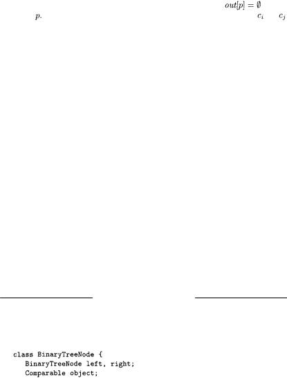
Fig. 4.4. Incremental construction of OFG edges for object sensitive analysis.

Fig. 4.4 shows the rules for OFG edge construction, when an object sensitive analysis is conducted. Some object scoped locations connected by OFG edges can be computed directly from the abstract syntax of the code under analysis. This happens when the scope of the location is the object allocated at the current statement or the object scoping the current method. Let us consider statement (5) in Fig. 4.4. The scope of the invoked constructor cs is

the currently allocated object	so that all formal parameters	as
well as the this location inside cs	will be scoped by

Class methods are replicated for each object of the given class allocated in the program. Inside such copies, a unique identifier of the current object (this) is available. It defines the scope of local variables, method parameters, and attributes of the current object.

The most difficult case is when an attribute is accessed or a method is called through a location other than this. In fact, in such a case, the target

70 4 Object Diagram

attribute or method belongs to an object other than the current one. If the attribute access has the form and the method call has the form the object scoping the related program locations is not directly available from the abstract statements. It can be obtained by executing the flow propagation algorithm for object analysis described in Section 4.2. However, such an algorithm requires the availability of the OFG, which has been built only partially. This is the reason why the rules in Fig. 4.4 have to be applied in-

crementally. During the first iteration of OFG construction,		for all
locations	Thus, only OFG edges connecting locations scoped by	or

(resp., the object allocated at current statement and the object scoping the current method) can be added to the OFG. Once this initial OFG is built, flow propagation for object analysis can be performed, giving a first estimate of the objects These objects can be used to scope the accesses to attributes of objects other than the current one, or method names and parameters, in case of an invocation to a target different from the current object. This allows adding more edges to the OFG, connecting locations scoped by an object different from the current one. The refined version of the OFG allows an improved estimation of the objects for each location thus possibly augmenting the set of edges added to the OFG, according to the rules in Fig. 4.4. At the end of this process, when no more edges are added to the OFG, the final, object sensitive OFG is obtained. OFG nodes will have out sets storing object identifiers determined through an object sensitive analysis. Thus, the object diagram derived from them is expected to be more accurate than the one constructed by an object insensitive analysis.

The algorithm described above produces quite precise object diagrams, since object flows are not mixed when they belong to the same class but to different objects. However, it requires replicating the program locations for all allocation sites, thus generating a larger OFG. Moreover, it assumes that the whole program is available for the analysis. In fact, if an allocation point for a class is not part of the code under analysis, some of the related edges in the OFG are missed, since will remain empty during all OFG construction iterations. In other words, the result of the object sensitive analysis is still safe (conservative) only if the whole system is available for the analysis, including all object allocation statements.

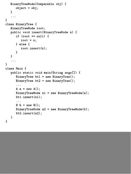
binary search tree example

Let us consider the following Java code fragment for a binary tree program. Two binary tree data structures, bt1 and bt2, are created to handle two different kinds of data elements: objects of class A and objects of class B.

4.3 Object Sensitivity

71

Fig. 4.5. Object insensitive OFG for object analysis.

Fig. 4.5 shows the object insensitive OFG built for the code fragment above. All program locations are scoped by the class they belong to. The out sets provided for some OFG nodes are those obtained after completing

72 4 Object Diagram

the flow propagation on the OFG. They will be used for the object diagram construction.

Fig. 4.6. Object sensitive OFG for object analysis.

Fig. 4.6 shows the corresponding object sensitive OFG. Program locations are replicated for all allocated objects of their class. During the first iteration of the OFG construction, performed according to the incremental rules in Fig. 4.4, the edges marked with an asterisk cannot be added to the graph. In fact, they are originated by the two invocations:

which have invocation targets different from this. According to rule 3 in Fig. 4.4, the objects scoping the method name and the formal parameters of the method are to be obtained respectively from out[Main.main.bt1] and out[Main.main.bt2], but both sets are initially empty. Consequently, an OFG is built with missing edges, associated with these two calls (asterisks in Fig. 4.6).

4.3 Object Sensitivity

73

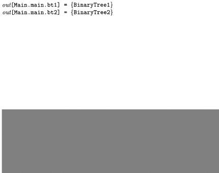
On the initial, partial OFG, the object analysis algorithm is run, and the result of the flow propagation at the two nodes of interest is:

This allows computing a proper scope for insert and its formal parameter n. Specifically, the invocation bt1.insert(n1) results in the addition of the two topmost edges marked with an asterisk in Fig. 4.6, since the target object of this invocation has been determined to be BinaryTree1 by the previous flow propagation step. Similarly, bt2. insert (n2) gives rise to the two asterisked edges at the bottom.

A new iteration of the flow propagation gives the final result of the object analysis. Some of the out sets obtained after this final flow propagation are shown in Fig. 4.6. They are exploited for the construction of the object diagram.

Fig. 4.7. Object diagram computed by an object insensitive analysis (left) and by an object sensitive analysis (right).

Object insensitive (Fig. 4.5) and object sensitive (Fig. 4.6) results are associated to the two object diagrams respectively on the left and on the right of Fig. 4.7. When object insensitive results are used for an object diagram construction, each class attribute is scoped by the class name, so that the relationships it induces are replicated for every object of that class. Thus, for example, the presence of BinaryTreeNode1 and BinaryTreeNode2 in the out set of BinaryTree. root originates the four associations labeled root in the object diagram on the left. Similarly, four associations labeled object are generated due to the output of BinaryTreeNode.object.

On the contrary, in the object sensitive OFG, class attributes are scoped by the object they belong to. Thus, the attribute root has two replications in Fig. 4.6, namely BinaryTree1.root and BinaryTree2.root, each with a different outset. Since only BinaryTreeNode1 is in the out of BinaryTree1.root, and only BinaryTreeNode2 is in the out of BinaryTree2.root, just two edges are constructed in the object diagram on the right for the associa-