140 7 Package Diagram

clusters have a feature vector that is coincident with that of the enclosed entity. Then, when a cluster contains feature vectors, its own feature vector is given by their sum: Thus, a cluster is associated to a feature vector with each coordinate given by the sum of the values of the same coordinate in all contained vectors.

Fig. 7.3. Clustering hierarchy (left), with two cut points selected, and associated package diagram (right).

When hierarchical clustering is applied for package diagram recovery, a partition of the classes can be obtained by cutting the hierarchy at an appropriate height (see Fig. 7.3). Successive cuts at different heights can be generated and assessed. Higher level cuts followed by lower level cuts indicate the cases where packages contain sub-packages. Lower level cuts eventually define packages that contain only classes.

With reference to Fig. 7.3, two cut points have been selected in the clustering hierarchy. The topmost cut defines a package containing two other packages, and a package containing 3 classes. The lower level cut in turn defines the content of the two packages that are merged at the higher level cut.

Problems that may occur when clustering is applied to software components, such as the classes, are the generation of a black hole, in which one cluster absorbs everything incrementally, while moving upward in the hierarchy, or, at the other extreme, the generation of a gas cloud, in which all singleton clusters tend to remain almost unchanged until the final grouping into a single final cluster [4]. Careful selection of the features to use, of the similarity measure between vectors and of the clustering algorithm to apply allow avoiding such problems.

7.2.2 Modularity Optimization

The approach to clustering based on modularity optimization [54] focuses on the relationships that hold among the entities to be clustered, rather than their features. In this setting, the goal of clustering is optimizing the level of

7.2 Clustering

141

modularity, so that the resulting grouping of the entities concurrently minimizes coupling (i.e., the connections between components of distinct clusters) while maximizing cohesion (i.e., the connections between components in a same cluster).

When this approach is applied to package diagram recovery, the relationships that hold among the classes have to be taken into account. The alternative choices span across those represented in the class diagram:

Inheritance.

Association.

Aggregation.

Composition.

Dependency.

All or a subset of them can be used for clustering. As discussed below, it may be important to be able to give different relationships different weights.

Given a set of entities (classes, in case of package diagram recover) and of relationships (inter-class relationships), cohesion and coupling can be formally defined as follows:

Cohesion:

Coupling:

where	is the number of relationships internal to cluster							is the num-
ber of relationships between clusters					and	and	is the number of
entities inside cluster			If auto-loops cannot occur in the relationships being
considered, the denominator of				becomes
	and	range between 0 and 1.			is 1 when the entities in cluster
are fully connected with each other					with auto-loops,
without auto-loops), while it is 0 when they are completely disconnected.
is equal to 1 when each entity of cluster					is	connected	to each entity		of
cluster	and	vice-versa.		is 0 when the entities in			and	have	no

connection with each other.

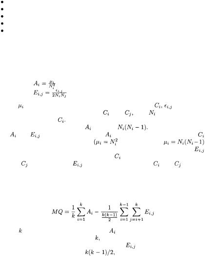
A joint measure of the modularization quality, MQ, can be obtained as the difference between the normalized total cohesion and the normalized total coupling:

where is the number of clusters. Since		is between 0 and 1, the sum over
all clusters will be between 0 and	hence the normalizing denominator of
the first term in MQ. As regards	the sum	of	over all pairs of different
clusters, the maximum will be		i.e., equal to the number of such

pairs. This number is used to normalize the second term in MQ, so as to make it range between 0 and 1.

142 7 Package Diagram

As a consequence of the normalization of the sums, MQ is bounded between -1 (no cohesion, maximum coupling) and 1 (no coupling, maximum cohesion). The latter situation is of course the most desirable one. Thus, the clustering algorithm based on the modularity metric MQ aims at determining the partition of the entities into clusters that maximizes MQ.

The problem of clustering has been turned into a combinatorial optimization problem. Consequently, the heuristics available from the field of combinatorial optimization can be used to approximate the optimal solution. The exact optimal solution is in general non computable, since the number of possible partitions for which MQ should be determined grows exponentially with the number of entities to be clustered.

Fig. 7.4. Hill-climbing clustering algorithm.

In the literature, several algorithms have been investigated to determine the clusters that maximize MQ [32, 54]. Fig. 7.4 shows a simple algorithm, based on the hill-climbing technique. It exploits the notion of neighbor partition. A partition NP is a neighbor of a partition P if it is the same as P except for a single element that belongs to different clusters in the two partitions. Initially, a random partition P is produced out of the set S of the entities to be clustered (line 2, Fig. 7.4). Then, an optimization loop is entered, which ends when the chosen strategy is unable to further improve the current partition of the entities. At line 4, a subset of all neighboring partitions, consisting of those with a higher MQ than P, is determined and assigned to BNP. If at least one better neighbor partition actually exists, P is reassigned (line 6). When more than one improvement directions are possible, one is chosen randomly. In the end, a (sub-)optimal partitioning of the entities is produced which can be interpreted as the package diagram being recovered from the inter-class relationships.

The main limitation of the algorithm in Fig. 7.4 is that its result is quite sensitive to the initial, random partition, from which optimization is started. This can be (partially) mitigated by executing it several times, starting from