74 4 Object Diagram

tion labeled root. Similarly, the output of BinaryTreeNode1.object and BinaryTreeNode2.object in the object sensitive OFG allows drawing the two associations labeled object in the object diagram on the right in Fig. 4.7.

The object diagram obtained by the object sensitive analysis conveys accurate information about the data elements stored in the two binary trees bt1 and bt2. In fact, node BinaryTreeNode1 has an attribute object that tpoints to A1, while BinaryTreeNode2 points to B1 (see Fig. 4.7, right). This indicates that the first tree is used to manage objects of class A (created at allocation point 1), while the second tree has a different purpose: managing objects allocated as B1. On the contrary, the object insensitive diagram is less accurate and does not allow distinguishing the data elements stored in the two trees.

Both object diagrams in Fig. 4.7 are safe, that is, they represent a conservative superset of all inter-object relationships that may occur at run time. However, the object sensitive one is more precise. The object insensitive diagram contains spurious associations, but has the advantage of being computable even when not all object allocations are part of the code under analysis.

4.4 Dynamic Analysis

The dynamic construction of the object diagram is achieved by tracing the execution of a target program on a set of test cases. The tracing facilities required are basically the possibility to inspect the current object and its attributes each time a method is invoked on an object and its statements are executed. Trace data should include an object identifier for the current object and for any object referenced by the current object’s attributes.

It is possible to obtain these dynamic data either by exploiting available tracing tools or by instrumenting the given program. In case of program instrumentation, the following additions are required:

Classes are augmented with an object identifier, which is computed and traced during the execution of class constructors.

Upon an attribute change, the identifier(s) of the object(s) referenced by the given attribute are added to the execution trace.

Time stamps are produced and traced when either of the two events above occurs.

Each program execution is thus associated with an execution trace, the analysis of which produces an object diagram. Consequently, the outcome of the dynamic analysis is a set of object diagrams, each associated with a test case, providing information on the objects and the relationships that are

4.4 Dynamic Analysis

75

instantiated in the test case. Their construction from the execution trace is straightforward. The identifier of each object in the execution trace is associated to a node in the dynamic object diagram. The identifiers of the objects referenced by the current object’s attributes determine the relationships between the current object and the other ones.

Since the relationship between two objects on a given attribute may change over time, if such an attribute is successively reassigned, in the execution trace multiple target objects may be associated to the same attribute at different times, resulting in more than one association to be drawn in the object diagram for that attribute. Their interpretation is that there exists a time interval when each drawn relationship actually holds. The traced time stamps are exploited when the dynamic object diagram is built, to decorate objects and associations with the time interval that represents their life span (from creation time to deletion time). Snapshots of the object diagram at a given time point or for a given interval can also be derived from the overall diagram.

binary search tree example

With reference to the binary tree example described in Section 4.3, let us assume that the tree is kept ordered according to the compareTo method available for the attribute object (inside class BinaryTreeNode), which implements the Comparable interface. A test case may consist in the creation of one or more BinaryTreeNode objects, with a String parameter assigned to the attribute object, and the insertion of the newly created node into a same BinaryTree. We can, for example, consider the following sequences of three strings as our test cases TC1, TC2, TC3. A node is created and inserted into the binary tree for each string encountered in the sequence:

TC1 ("a", TC2 ("b", TC3 ("c",

"b", "c") "a", "c") "b", "a")

76 4 Object Diagram

Fig. 4.8. Dynamic construction of object diagrams for test cases TC1, TC2 and

TC3.

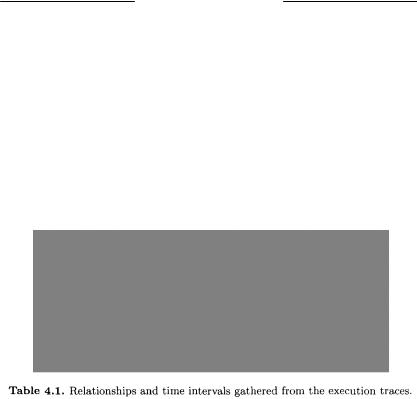
The execution traces for these three test cases contain the information in Table 4.1 (attributes with null value have been removed from the execution trace, being not relevant for the construction of the object diagram). Time intervals in which a given relation holds are given in square brackets.

The analysis of the three execution traces produces the three object diagrams depicted in Fig. 4.8. In TC1, all child nodes are added on the right. In TC2, the tree is balanced, while in TC3 only left children are present. The life span of objects and relationships is in square brackets.

4.4.1 Discussion

Static extraction and dynamic extraction of the object diagram produce different but complementary information about the instantiations of the classes performed by a program. The static object diagram gives a conservative view of the objects that are possibly created by the program and of the relationships that may exist between the objects. The number of objects reflects the number of program locations where an allocation statement is present. If such a statement is executed multiple times, the actual multiplicity of the related object is greater than the multiplicity indicated in the static object diagram (i.e., one). The presence of a relationship between two objects in the static object diagram indicates that there is some path in the program along which the first object may reference the second one (through some of its attributes). The existence of a path in the program does not imply that such a path is traversed in every execution. As a consequence, the relationships between

4.4 Dynamic Analysis

77

objects indicated in the static object diagram are a conservative superset of those actually instantiated at run time. Moreover, it may happen that some of these relationships are associated to paths that can never be followed, for any input value. This is typical of static analysis: the solution is conservative, but may include infeasible parts, due to mutually exclusive conditions on the input values.

The dynamic object diagram complements the static one, in that objects are replicated in it each time a same allocation statement is re-executed, thus giving a better picture of their actual multiplicity. However, such a diagram is always partial, being based on a limited and necessarily incomplete set of test cases. An indication of the parts of the object diagram not yet explored can be obtained by contrasting it with the static object diagram. Objects and relationships in the static object diagram that are not represented in the dynamic one are associated respectively to allocation statements and execution paths not exercised by the available test cases.

binary search tree example

As depicted in Fig. 4.3 (right), the binary tree example has a static object diagram with 4 nodes and 7 edges. The first test case executed on it (Fig. 4.8, TC1) instantiates its objects in 3 out of the 4 locations identified statically. Allocation of a BinaryTreeNode in case of left insertion (addLeft) is not exercised in TC1. Consequently, the two edges leaving BinaryTreeNode2 in the static object diagram and the two incoming edges are not represented in the first dynamic object diagram. However, the first dynamic object diagram provides some additional information on the multiplicity of the object