Ersoy O.K. Diffraction, Fourier optics, and imaging (Wiley, 2006)(ISBN 0471238163)(427s) PEo

8	LINEAR SYSTEMS AND TRANSFORMS

where a1 and a2 are scalars. Above ðx; yÞ is replaced by ½m; n& in the case of a linear discrete-space system.

Suppose that the input at ðx1; y1Þ is the delta function d(x1, y1) (see Appendix A for a discussion of the delta function). The output at location ðx; yÞ is defined as

hðx; y; x1; y1Þ ¼ O½dðx x1; y y1Þ&

ð2:2-4Þ

hðx2; y2; x1; y1Þ is called the impulse response (point-spread function) of the system. The sifting property of the delta function allows an arbitrary input uðx; yÞ to be

expressed as

	1
uðx; yÞ ¼	ð ð uðx1; y1Þdðx x1; y y1Þdx1dy1	ð2:2-5Þ
	1

Now the output can be written as

gðx; yÞ ¼ O½uðx; yÞ&

ð1 ð

¼uðx1; y1ÞO½dðx x1; y y1Þ&dx1dy1

1 ð2:2-6Þ

1ð

¼uðx1; y1Þhðx; y; x1; y1Þdx1dy1

1

This result is known as the superposition integral. Physically, the delta function corresponds to a point source. The superposition integral implies that all we need to know is the response of the system to point sources throughout the field of interest in order to characterize the system.

A linear imaging system is called space invariant or shift invariant if a translation of the input causes the same translation of the output. For a point source at the origin, the output of a shift-invariant system can be written as

hðx; y; 0; 0Þ ¼ O½dðx; yÞ&

ð2:2-7Þ

If the input is shifted as dð x1; y1Þ, the output of the shift-invariant system must be hðx x1; y y1; 0; 0Þ. This is usually written simply as

hðx; y; x1; y1Þ ¼ hðx x1; y y1Þ		ð2:2-8Þ
Then, the superposition integral becomes
	1
gðx; yÞ ¼	ð ð uðx1; y1Þhðx x1; y y1Þdx1dy1	ð2:2-9Þ
	1

LINEAR SYSTEMS AND SHIFT INVARIANCE

9

By a change of variables, this can also be written as

	1	ð hðx1; y1Þ f ðx x1; y y1Þdx1dy1
gðx; yÞ ¼	ð		ð2:2-10Þ
	1

This is the same as the 2-D convolution of hðx; yÞ with uðx; yÞ to yield gðx; yÞ. It is often written symbolically as

gðx; yÞ ¼ hðx; yÞ uðx; yÞ

ð2:2-11Þ

The significance of this result is that a linear shift-invariant (LSI) system is governed by convolution. Hence, the convolution theorem can be used to express the input–output relationship as

Gðfx; fyÞ ¼ Hð fx; fyÞUð fx; fyÞ

ð2:2-12Þ

where Gð fx; fyÞ, Hð fx; fyÞ, and Uð fx; fyÞ are the Fourier transforms of gðx; yÞ; hðx; yÞ and uðx; yÞ, respectively. The Fourier transform is discussed in the next section. Hð fx; fyÞ given by

	1	ð hðx; yÞe j 2pð fxxþfyyÞdxdy;
Hð fx; fyÞ ¼	ð		ð2:2-13Þ
	1

is called the transfer function of the system.

In the case of a discrete-space system, the superposition integral becomes the superposition sum, given by

1	1
X	X	ð2:2-14Þ
g½m; n& ¼	u½m1; n1&h½m; n; m1; n1&

m1¼ 1 n1¼ 1

In the case of a discrete-space LSI system, the convolution integral becomes the convolution sum, given by

1	1
X	X	ð2:2-15Þ
g½m; n& ¼	u½m1; n1&h½m m1; n n1&;

m1¼ 1 n1¼ 1

which can also be written as

1	1
X	X	ð2:2-16Þ
g½m; n& ¼	h½m1; n1&u½m m1; n n1&

m1¼ 1 m2¼ 1

10	LINEAR SYSTEMS AND TRANSFORMS

The transfer function of a discrete-space LSI system is the discrete-space Fourier transform of the impulse response, given by

X	X
1	1	ð2:2-17Þ
Hð fx; fyÞ ¼	h½m1; n1&e j 2pð fxm1 xþf2n1 yÞ

m1¼ 1 n1¼ 1

The convolution theorem is stated by Eq. (2.2-12) in this case as well.

2.3CONTINUOUS-SPACE FOURIER TRANSFORM

The property of linearity allows the decomposition of a complex signal into elementary signals often called basis signals. In Fourier analysis, basis signals or functions are sinusoids.

The 1-D Fourier transform of a signal uðtÞ, 1 t 1 is defined as

	1
Ucðf Þ ¼	ð	uðtÞe j 2p ftdf	ð2:3-1Þ
	1

The inverse Fourier transform is the representation of uðtÞ in terms of the basis functions e j2pft and is given by

	1
uðtÞ ¼	ð	Ucð f Þe j2p ftdf	ð2:3-2Þ
	1

Equation (2.3-1)is also referred to as the analysis equation. Equation (2.3-2) is the corresponding synthesis equation.

The multidimensional (MD) Fourier transform belongs to the set of separable unitary transforms as the transformation kernel is separable along each direction. For example, the 2-D transform kernel bðx; y; fx; fyÞ can be written as

bðx; y; fx; fyÞ ¼ b1ðx; fxÞb2ðy; fyÞ

ð2:3-3Þ

bið ; Þ for i equal to 1 or 2 is the 1-D transform kernel.

The 2-D Fourier transform of a signal uðx; yÞ, 1 < x; y < 1 is defined as

	1
Uðfx; fyÞ ¼	ð ð uðx; yÞe j2pðxfxþyfyÞdxdy;	ð2:3-4Þ
	1

where fx and fy are the spatial frequencies corresponding to the x- and y-directions, respectively.

EXISTENCE OF FOURIER TRANSFORM

11

The inverse transform is given by

	1	ð Uð fx; fyÞe j2pðxfxþyfyÞdfxdfy
uðx; yÞ ¼	ð		ð2:3-5Þ
	1

2.4EXISTENCE OF FOURIER TRANSFORM

Sufficient conditions for the existence of the Fourier transform are summarized below:

A.The signal must be absolutely integrable over the infinite space.

B.The signal must have only a finite number of discontinuities and a finite number of maxima and minima in any finite subspace.

C.The signal must have no infinite discontinuities.

Any of these conditions can be weakened if necessary. For example, a 2-D strong, narrow pulse is often represented by a 2-D impulse (Dirac delta) function, defined by

dð	x; y	Þ ¼	lim N2e N2pðx2þy2Þ		ð	2:4-1	Þ
			N	!1

This function fails to satisfy condition C. Two other functions that fail to satisfy condition A are

uðx; yÞ ¼ 1

ð2:4-2Þ

uðx; yÞ ¼ cos 2pfxx

With such functions, the Fourier transform is still defined by incorporating generalized functions such as the delta function above and defining the Fourier transform in the limit. The resulting transform is often called the generalized Fourier transform.

EXAMPLE 2.1 Find the FT of the 2-D delta function, using its definition.

Solution: Let

uðx; yÞ ¼ N2e N2pðx2þy2Þ

Then,

dðx; yÞ ¼ lim f ðx; yÞ

N!1

12	LINEAR SYSTEMS AND TRANSFORMS

Now, we can write

Uðfx; fyÞ ¼ e pð fx2þfy2Þ=N2

Denoting ðfx; fyÞ as the Fourier transform of dðx; yÞ in the limit as N ! 1, we find

ðfx; fyÞ ¼ lim Uð fx; fyÞ ¼ 1

N!1

2.5PROPERTIES OF THE FOURIER TRANSFORM

The properties of the 2-D Fourier transform are generalizations of the 1-D Fourier transform. We will need the definitions of even and odd signals in 2-D. A signal uðx; yÞ is even (symmetric) if

uðx; yÞ ¼ uð x; yÞ

(2.5-1)

uðx; yÞ is odd (antisymmetric) if

uðx; yÞ ¼ uð x; yÞ

(2.5-2)

These definitions really indicate two-fold symmetry. It is possible to extend them to four-fold symmetry in 2-D.

Below we list the properties of the Fourier transform.

Property 1: Linearity

If gðx; yÞ ¼ au1ðx; yÞ þ bu2ðx; yÞ, then
Gð fx; fyÞ ¼ aU1ð fx; fyÞ þ bU2ð fx; fyÞ	ð2:5-3Þ
Property 2: Convolution
If gðx; yÞ ¼ u1ðx; yÞ u2ðx; yÞ, then
Gð fx; fyÞ ¼ U1ð fx; fyÞU2ð fx; fyÞ	ð2:5-4Þ

Property 3: Correlation is similar to convolution, and the correlation between u1ðx; yÞ and u2ðx; yÞ is given by

gðx; yÞ ¼ ðð u1ðx1; y1Þu2ðx þ x1; y þ y1Þdx1dy1	ð2:5-5Þ
1
1
If gðx; yÞ ¼ u1ðx; yÞ u2ðx; yÞ, where denotes 2-D correlation, then
Uð fx; fyÞ ¼ U1ð fx; fyÞU2 ð fx; fyÞ	ð2:5-6Þ

PROPERTIES OF THE FOURIER TRANSFORM						13
Property 4: Modulation
If gðx; yÞ ¼ u1ðx; yÞu2ðx; yÞ, then
Gð fx; fyÞ ¼ F1ð fx; fyÞ F2ð fx; fyÞ						ð2:5-7Þ
Property 5: Separable function
If gðx; yÞ ¼ u1ðxÞu2ðyÞ, then
Gð fx; fyÞ ¼ U1ð fxÞU2ð fyÞ						ð2:5-8Þ
Property 6: Space shift
If gðx; yÞ ¼ uðx x0; y y0Þ, then
Gð fx; fyÞ ¼ e j2pð fxx0þfyy0Þ Uð fx; fyÞ						ð2:5-9Þ
Property 7: Frequency shift
If gðx; yÞ ¼ e j2pð fx0xþfy0yÞ uðx; yÞ, then
Gð fx; fyÞ ¼ Uð fx fx 0; f2 fy 0Þ						ð2:5-10Þ
Property 8: Differentiation in space domain
If gðx; yÞ ¼ @k=@xk @‘=@y‘ uðx; yÞ, then
Gð fx; fyÞ ¼ ð2p jfxÞkð2p jfyÞ‘Uð fx; fyÞ						ð2:5-11Þ
Property 9: Differentiation in frequency domain
If gðx; yÞ ¼ ð j2pxÞkð j2pyÞ‘uðx; yÞ, then
		@k @‘
Gð fx; fyÞ ¼					Uð fx; fyÞ	ð2:5-12Þ
		@fxk		@fy‘
Property 10: Parseval’s theorem
1	1	ð Uð fx; fyÞG ð fx; fyÞdfxdfy
ð ð uðx; yÞg ðx; yÞdxdy ¼	ð					ð2:5-13Þ
1	1
Property 11: Real uðx; yÞ
Uð fx; fyÞ ¼ U ð fx; fyÞ						ð2:5-14Þ

Property 12: Real and even uðx; yÞ

Uð fx; fyÞ is real and even

14							LINEAR SYSTEMS AND TRANSFORMS
Property 13: Real and odd uðx; yÞ
			Uð fx; fyÞ is imaginary and odd
Property 14: Laplacian in the space domain
@2			@2
If gðx; yÞ ¼		þ		uðx; yÞ, then
	@x2		@y2
			Gð fx; fyÞ ¼ 4p2ð fx2 þ fy2ÞUð fx; fyÞ						ð2:5-15Þ
Property 15: Laplacian in the frequency domain
If gðx; yÞ ¼ 4p2ðx2 þ y2Þuðx; yÞ, then
			Gð fx; fyÞ ¼		@2	þ	@2	!Uð fx; fyÞ	ð2:5-16Þ
					@fx2		@fy2
Property 16: Square of signal
If gðx; yÞ ¼ juðx; yÞj2, then
			Gð fx; fyÞ ¼ Uð fx; fyÞ U ð fx; fyÞ						ð2:5-17Þ
Property 17: Square of spectrum
If gðx; yÞ ¼ uðx; yÞ u ðx; yÞ, then
				Gð fx; fyÞ ¼ jUð fx; fyÞj2					ð2:5-18Þ
Property 18: Rotation of axes
If gðx; yÞ ¼ uð x; yÞ, then
				Gð fx; fyÞ ¼ Uð fx; fyÞ					ð2:5-19Þ

The important properties of the FT are summarized in Table 2-1.

EXAMPLE 2.2 Find the 1-D FT of

1ð

gðxÞ ¼

uðx; yÞdy

1

as a function of the FT of uðx; yÞ.

PROPERTIES OF THE FOURIER TRANSFORM

15

Table 2.1. Properties of the Fourier transform (a, b,

fx0

and fy0

are real nonzero

constants; k and l are nonnegative integers).

Property

gðx; yÞ

Gðfx; fyÞ

Linearity

au1ðx; yÞ þ bu2ðx; yÞ

aU1ð fx; fyÞ þ bU2ð fx; fyÞ

Convolution

u1ðx; yÞ u2ðx; yÞ

U1ð fx; fyÞU2ð fx; fyÞ

Correlation

u1ðx; yÞ u2ðx; yÞ

U1ð fx; fyÞU2 ð fx; fyÞ

Modulation

u1ðx; yÞu2ðx; yÞ

U1ð fx; fyÞ U2ð fx; fyÞ

Separable function

u1ðxÞu2ðyÞ

U1ð fxÞU2ð fyÞ

Space shift

uðx

x0; y y0Þ

e

j2pð fxx0þfy y0 Þ Uð fx; fyÞ

Frequency shift

gðx; yÞ ¼ e j2pð fx0xþfy0yÞ uðx; yÞ

Gð fx; fyÞ ¼ Uð fx

fx0; f2

fy0Þ

@k

@‘

ð2pjfxÞkð2pjfyÞ‘Uð fx; fyÞ

Differentiation in

uðx; yÞ

@xk

@y‘

space domain

@k

@‘

ð j2pxÞkð j2pyÞ‘uðx; yÞ

Differentiation in

Uð fx; fyÞ

@f k

@f ‘

frequency domain

@2

@2

x

y

Laplacian in the space

2

2

2

@x2 þ @y2

uðx; yÞ

4p ð fx

þ fy ÞUð fx; fyÞ

domain

Laplacian in

4p2ðx2 þ y2Þuðx; yÞ

@2

þ

@2

!Uð fx; fyÞ

@fx2

@fy2

the frequency domain

Square of signal

j

ð

Þj

2

U

ð

fx

; fy

Þ

U

ð

fx; fy

Þ

u x; y

Square of spectrum

uðx; yÞ u ðx; yÞ

jUð fx; fyÞj2

Rotation of axes

1

uð x; yÞ

1

Uð fx; fyÞ

ð Uð fx; fyÞG ð fx; fyÞdfxdfy

Parseval’s theorem

ð ð uðx; yÞg ðx; yÞdxdy ¼

ð

1

1

Real uðx; yÞ

Uð fx; fyÞ ¼ U ð fx;

fyÞ

Real and even uðx; yÞ

Uð fx; fyÞis real and even

Real and odd uðx; yÞ

Uð fx; fyÞis imaginary and odd

Solution: gðxÞ and dðxÞ are considered as 2-D functions gðxÞ 1 and dðxÞ 1, respectively. Then, gðxÞ can be written as

gðxÞ 1 ¼ uðx; yÞ ½dðxÞ 1&			xÞdx1dy1
¼	ðð	uðx1; y1Þdðx1
	1
	1
	1
¼	ð	uðx; yÞdy	ð2:5-20Þ

1

16	LINEAR SYSTEMS AND TRANSFORMS

Computing the FT of both sides of Eq. (2.5-20) and using the convolution theorem and property 5 of separable functions gives

Gð fxÞdð fyÞ ¼ Uð fx; fyÞdð fyÞ

or

Gð fxÞ ¼ Uð fx; 0Þ

EXAMPLE 2.3 Find the FT of

gðx; yÞ ¼ uða1x þ b1y þ c1; a2x þ b2y þ c2Þ

as a function of the Fourier transform of uðx; yÞ.

Solution:

ðð uða1x þ b1y þ c1; a2x þ b2y þ c2Þe j2pð f1xþf2yÞdxdy

Gð fx; fyÞ ¼

1

1

Letting x1 ¼ a1x þ b1y þ c1 gives

1

þ b2y þ c2 e j2p fx

a1 þfyy

ja11j

Gð fx; fyÞ ¼

ðð u x1; a2 x1

a11

1

b y

c

x1 a1y c1

dx dy

1

1 ¼

a

2

a1

þ

b

2

y

þ

c

2

gives

Also letting y

x1 b1y c1

Gðfx; fyÞ ¼ jDj

ðð

uðx1; y1Þe j2p½x1fx0 þy1fy0 þT1fxþT2fy&dx1dy1

ð2:5-21Þ

1

1

1

where

D ¼ a2b1 a1b2

fx0 ¼ D1 ð a1fx þ a2fyÞ

fy0 ¼ 1 ðb1fx a1fyÞ D

T1 ¼ b1c2 b2c1

D

T2 ¼ a2c1 a1c2

D

PROPERTIES OF THE FOURIER TRANSFORM

17

Equation (2.5-21) is the same as

Gðfx; fyÞ ¼ j1j e j2pðT1 fxþT2 fyÞUð fx0; fy0Þ

D

In other words, when the input signal is scaled, shifted, and skewed, its transform is also scaled, skewed, and linearly phase-shifted, but not shifted in position.

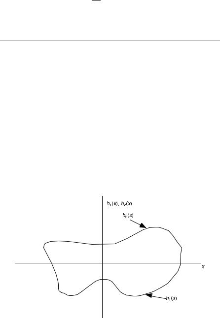
EXAMPLE 2.4 Find the FT of the ‘‘one-zero’’ function defined by

u x; y	Þ ¼	1	h1ðxÞ < y < h2	x	Þ	;
ð		0	otherwise	ð

where h1ðxÞ and h2ðxÞ are given single-valued functions of x. Determine Uðfx; fyÞ and Uðfx; 0Þ.

Solution: uðx; yÞ is as shown in Figure 2.2. Its FT is given by

ðð1

Uðfx; fyÞ ¼ uðx; yÞe j 2pð fxxþfyyÞdxdy

1

1ð h2ðxÞ

¼	e j 2p fx xdx	e j 2p fy ydy

1 h1ðxÞ

Figure 2.2. A typical zero-one function.