Emerging Tools for Single-Cell Analysis

294	White-Light Scanning Digital Microscopy

white raster pattern on its screen. This pattern is imaged through a microscope relay lens and objective lens onto the sample placed on the microscope stage.

The size of the raster image on the sample is determined by the lens system magnification. For example, an ordinary microscope may have a 40-power objective lens and a 10-power eyepiece lens, giving a combined magnification of 400 from the sample to the eye. Operated in reverse, an object placed outside the eyepiece lens will be demagnified 400 times down to the sample plane.

This one-to-one mapping of the scanning spot from the CRT screen onto the sample plane creates a tiny white probe in a dark field that scans over the sample. The spot characteristics on the sample are completely determined by the microscope objective. As a result, the probing spot has the smallest diffraction-limited diameter possible for each objective lens.

The light transmitted through the sample is divided by dichroic mirrors into red (580–650 nm), green (520–580 nm), and blue (450–520 nm) spectral components and passed to three detectors. A video display reconstructs the image of the sample using the x–y position of the scanning spot and the three color intensities. In the simplest case, the scan frequency of the CRT raster matches the scan frequency of the display, giving a direct correspondence between the spot position on the CRT and the spot position on the display.

DETECTION SYSTEM

The detectors in this digital microscope are not the CCD imaging devices used in most “digital” cameras today. Instead, the detectors are three nonimaging photomultiplier tubes (PMTs) that collect the intensity signals simultaneously in the three spectral bands. Color registration is inherently perfect since there is only one spot scanning over the sample and the PMT detectors read intensity only in the color bands. The PMTs used are ordinary types available from several manufacturers, capable of achieving full color saturation with signals of less than 100 nW of power. More expensive or cooled PMT detectors could be used for special applications.

SIGNAL PROCESSING

Performance can be improved by reducing the scan frequency of the CRT well below the scan frequency of the display. The data are read in at one rate, then presented to the display at a faster rate. The choice of scan rate at the sample is determined by the number of pixels in the image and the desired optical contrast function. From a purely technical standpoint, the number of pixels in the digital image could be chosen as any value, but practical considerations of the data file size, availability of displays, processing and transmission times, and correlation with direct viewing set reasonable boundaries to the image file size.

Signal Processing

295

F i g . 13.2. Signal processing path showing how the transmitted light is handled for each spectral channel.

These considerations led to the choice of image size for COSMIC as 1280 1024 pixels with 24 bits/pixel color depth. Displays are readily available for this resolution and the data set is manageable for computation, storage, and transmission. The image size is a reasonable match to the number of optical resolution elements in various microscope images as viewed directly by the eye. The selected frame rate of 13.4 Hz is fast enough to observe live cells. The resulting data rate is 420 Mbits/s, which is at the high end of current imaging technologies.

Figure 13.2 illustrates the electronic signal path. The three color signals from the detectors are amplified and sent to a digital imaging board that performs multiple functions. First, the three signals are digitized into parallel 1280 1024 math buffers. The data in the three math buffers are transferred to three display buffers, converted into analog signals, and sent to the display at a 60-Hz frame rate. Math

296	White-Light Scanning Digital Microscopy

functions for averaging up to 256 images and summing (integrating) up to 9999 images are executed in the math buffers by programming built into the imaging board. These functions operate at the full frame rate.

ZOOM MAGNIFICATION

The optical magnification can be changed instantaneously up to 300% (3 ) by changing the scanned area on the sample. The principle is illustrated in Figure 13.3. The scan raster overlaying the sample is shown on the left and the resulting image on the display is shown on the right. The image is always digitized into 1280 1024 pixels, so the data set remains constant for any magnification, and the pixel size never changes within the field of view.

Operating an objective lens at three times its rated magnification will exceed its classical resolution limit, resulting in so-called empty magnification, which has tra-

F i g . 13.3. As the scan area decreases, the specimen fills more of the image window. The display area is constant in size, thus the specimen is enlarged. The image is always digitized at 1280 1024 data points, creating a constant file size at all zoom values.

Brightness and Focus Change

297

F i g . 13.4. Example of a zoomed image. Here, a mosquito head is imaged using the microscopes 10x objective with no zoom (A), zoom at 1.5x (B), and zoom at 3x (C). See color plates.

ditionally been considered a useless exercise. However, what really happens is that each optical resolution element may be digitized into as many as six data points, resulting in a process called digital oversampling. Oversampling tends to push resolution limits beyond standard conventions and results in “superresolution.” Oversampling is discussed in more detail below.

The zoom feature also reduces the need for larger digital image files having more pixels since one can instantaneously zoom in to display maximum resolution at reduced field size. COSMIC’s constant file size means that transmission times are invariant for all images. Figure 13.4 shows an example of a zoomed image. Here, a mosquito head is imaged using COSMIC’s 10x objective with no zoom (A), zoom at 1.5 (B), and zoom at 3 (C).

BRIGHTNESS AND FOCUS CHANGE

Some unexpected characteristics occur with the zoom capability. In an ordinary optical zoom lens two things happen when the field size is changed. The brightness changes because the numerical aperture (NA) has changed (the change in focal length changes the NA), and the focus changes because it is virtually impossible to make a variable-focus lens with moving parts that can maintain constant focus throughout its range. In a point scanning microscope, on the other hand, the zoom feature does not change the focus or the brightness, which are not simply constants but universal constants. The focus does not change because mechanical distances are fixed. There are no alterations in the distance between the lenses and image planes at any time. The changes are related only to the area scanned on the sample. The size of the scanned area has been decreased, but all the mechanical distances remain the same. Another important characteristic of the zoom feature is that the brightness does not change. The illumination energy density on the sample varies with the size of the scanned area. For a large area, the energy per unit area is low. This is because the illumination emitted by the CRT is constant. Only the scanned area changes and therefore the energy density changes linearly with area.

The change in brightness between two different illumination areas can be shown mathematically to be inversely proportional to the ratio of the areas. Since the illumi-

298	White-Light Scanning Digital Microscopy

nation on the sample changes proportionally to the area ratio, the brightness in the final image does not change with zoom.

CONTRAST ENHANCEMENT AND SUPPRESSION

In other spot-scanning instruments, such as laser scanning microscopes and electron beam microscopes, the intensity of the spot is constant as it scans over the sample. With COSMIC, however, it is possible to modulate the brightness of the spot for every pixel in the sample plane. If the spot is modulated using data from the sample, then several interesting effects are possible. Figure 13.5A illustrates the usual condition of a con- stant-intensity scan overlaid on the sample and the resultant image on the display. In Figure 13.5B, the CRT raster has a positive image of the sample superimposed on it. When transferred to the sample plane, the spot goes bright when the sample is bright

F i g . 13.5. Concepts of spot modulation demonstrated. The brightness of the scanning spot is varied point by point as it traces over the sample in order to increase or decrease the light/dark signal swing. Three effects are shown: standard (A), contrast enhancement (B), and contrast suppression (C).

Averaging and Summing

299

F i g . 13.6. Image enhancement features of COSMIC. The normal-mode image of Figure 4 (A), the image in contrast suppression mode (B), and the image in color-inverted mode (C). This mode is particularly useful to identify thin structures in cells where the color inversion highlights the objects. See color plates.

and dark when the sample is dark, resulting in increased contrast in the image on the display. If the CRT has a negative image superimposed on it (Figure 13.5C), then the spot is dark when the sample is bright and bright when the sample is dark, suppressing contrast in the image. The contrast enhancement feature is very useful for examining unstained samples, and contrast suppression is useful for overstained or dark samples. Many of these samples cannot be successfully imaged with conventional microscopes. Figure 13.6 (A) is the same normal-mode sample as Figure 4. Figure 13.6 (B) demonstrates the contrast enhancement due to spot modulation, and Figure 13.6 (C) shows digital color inversion.

RESPONSE FUNCTION

Most television imaging and display tubes have a nonlinear response represented by an exponential equation using the variable “gamma.” Gamma correction circuits are used routinely in video amplifiers to linearize the response.

Although the response function of the digital microscope is inherently linear, a programmable response function has been designed into the imaging board. In terms of gray-level histograms, spot modulation expands or compresses the whole histogram, while the gamma can adjust the midlevel values and not the end points. The gamma response function and spot modulation functions can be used together to fine tune the desired image enhancement effects.

In addition to the modes discussed, digital brightness, contrast, and background correction can be applied. The presence of these functions recognizes the need for simple, real-time image processing, which reduces the need for postprocessing and ensures that the image saved is of the highest quality.

AVERAGING AND SUMMING

In order to boost weak and smooth noisy signals, two digital processing modes have been implemented in hardware using the math buffer. The averaging mode performs a running average of up to 256 images in steps of 2n, where n 1, . . . , 8. It is also possible to sum (or integrate) up to 9999 images. The summation mode not only reduces random noise in the final image by the square root of n but also acts as a gain

300	White-Light Scanning Digital Microscopy

factor up to 9999 for weak signals. The summed image can also be divided by powers of two as high as 256, giving a variable-gain factor. The summing mode is therefore a combination of gain and averaging and is particularly useful for very low signal levels. Both the averaging and summing modes operate at 13.4 frames per second. The new image creation rate is the number of frames processed divided by the system frame rate. For an averaging level of 2, therefore, new images appear at 6.7 Hz, and summing eight frames takes 0.60 s.

COMMUNICATIONS

The light scanning microscope has a SCSI port to save images to any kind of hard drive or removable drive. The file format is TIFF, a universal standard compatible with most image processing programs. An ethernet port is included for connection to networks for storage, archiving, and communication across the Internet or other telecommunication systems.

Files that have been created or modified in TIFF format by image processing or desktop publishing programs can be read back into COSMIC and shown on the display for teaching or conferences. A “slide show” mode can sequentially display all the images on the disk, so this means that text slides or photographs can be displayed along with the microscope images.

OVERSAMPLING AND SUPERRESOLUTION

As mentioned earlier, oversampling is a process of collecting more electronic data points than actually exist in the optical image. If there are 1000 optical resolution elements in a scan line across the image, and that line is digitized into 3000 data points, then that is oversampling. The number of optical resolution elements in a field of view can easily be calculated by using the classical Airy disk formula

0.61

R

o NA

where is the wavelength, typically chosen as 550 nm, and NA is the numerical aperture of the objective. According to the Rayleigh resolution criterion, Ro is the minimum distance resolvable by a lens with a given numerical aperture. It is also the radius of the Airy disk, which is the smallest dot that can be imaged by an objective, and will be referred to as the Airy disk size or the optical resolution element size.

Figure 13.7 shows a 40x objective with a numerical aperture of 0.75 which has an Airy disk size of 0.447 m that defines its resolution. In a normal field of view of diameter 500 m, there are approximately 1100 optical resolution elements across the center of the field. The COSMIC CRT raster scans a 3:4 aspect ratio rectangle whose diagonal is 70% of the 500- m circle diameter, resulting in a scanned area that is approximately 280 210 m, or about 626 470 Airy disks.

Oversampling and Superresolution

301

F i g . 13.7. A 40x objective with a NA of 0.75 has an Airy disk size of 0.447 m that defines its resolution. In a normal field of view of diameter 500 m, there are approximately 1100 optical resolution elements across the center of the field. The CRT raster scans a 3 : 4 aspect ratio rectangle whose diagonal is 70% of the 500- m circle diameter, resulting in a scanned area that is approximately 280 210 m, or about 626 470 Airy disks.

In order to determine the resolving power of the imaging system, it is necessary to take into account the sampling theory of Nyquist, who derived the number of samples needed to define a single point of a data curve. In terms of optics, to represent the information in a single optical resolution element (Airy disk), one must take two samples across the element. This is not really oversampling but adequate sampling, since 2 : 1 is the ratio needed for accurate sampling. Oversampling would therefore be anything over the 2 : 1 ratio. Examining Figure 13.7 again, it can be seen that for the 40x objective (with no zoom) 1280 points are digitized across the 626 Airy disks. The sampling ratio is right at 2:1, and it is reasonable to say that the data from the 40x objective are “just resolved.”

When the 40x field of view is zoomed by 3x, the number of optical resolution elements in the scanned area is reduced to 218 156, but the data are still digitized into 1280 1024 data points. This is almost a 6 : 1 oversampling (Plasek et al., 1998). In reality, oversampling does give an improved image over “adequate sampling”; that is, the modulation transfer function improves up to a certain point, after which there is no improvement. The image detail increases with magnification up to a point, after which the image gets larger but no more detail is seen (“empty magnification”).

Each objective power has a different number of optical resolution elements within the field of view. Interestingly, lower power objectives have more elements across the field of view, posing a greater imaging challenge than high-power objectives. For example, a 2.5x objective has a scanned area of 4.300 3.225 mm that contains

302		White-Light Scanning Digital Microscopy
A		B

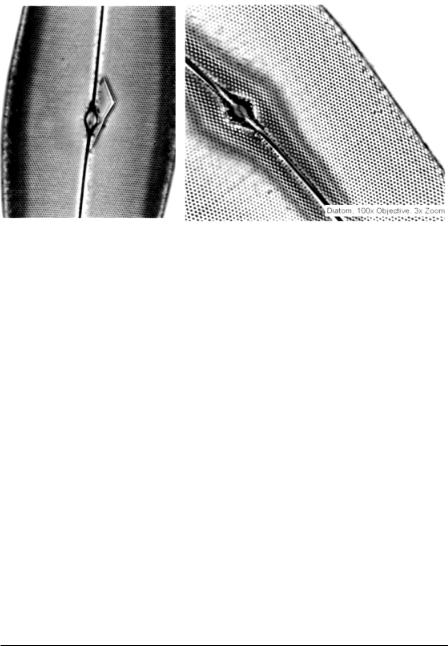
F i g . 13.8. Superresolution effect is demonstrated with an image of the diatom Pleurasigma angulatum. The holes in the diatoms are approximately 0.25 m in diameter and hexagonal in shape. The full-color images were taken in white light. Obtaining such high-resolution images is very difficult with most other systems. Figure 13.8 (A) was taken with a 40x (0.75NA) objective. Figure 13.8 (B) was taken with a 100x (1.3NA oil) objective. However, the sample is in air under the cover slip, so the maximum usable NA for the 100x objective is less than 1.0. The condensor had an NA of 1.4 (oil). See color plates.

961 721 Airy disks. The 1280 1024 electronic data points are less than the 2 : 1 ratio needed to fully resolve the smallest element in the image. However, if the image is zoomed by 1.6, the scanned area covers 600 400 Airy disks and all points in the field are fully resolved. The zoom control provides a convenient mechanism to trade field of view for full resolution whenever desired. Because the zoom factor will carry any objective into true empty magnification, the system resolution is limited by the objective’s ability to create an Airy disk, not the ability to take the data from it. Therefore, it is reasonable to say that the limit of resolution of this digital microscope is the optics, not the electronics.

This color scanning microscope can also exhibit superresolution, where image detail far smaller than the calculated limit has been observed. The technique uses the oversampling feature coupled with COSMIC’s summing, averaging, and background correction functions. Diatom images taken with a 40x objective (0.75 NA) have shown features as small as 0.05 µm, well below the Airy disk size of 0.447 µm. This superresolution effect is demonstrated in Figure 13.8, where an image is shown of Pleurasigma angulatum. The holes in these diatoms are approximately 0.25 m in diameter and are hexagonal in shape.

BRIGHTNESS AND COLOR CALIBRATION

The light transmitted through different objectives varies with the power of the objective. Significantly more light is transmitted through the 2.5x objective than through the 100x objective. In addition, the color balance of each objective is different, so the variation in red/green/blue balance must also be corrected. Calibration of brightness and

Comparison with Camera Systems

303

color balance to standard values is done by adjusting the gain setting of each PMT detector for each objective. A sensor embedded in the objective nose piece automatically selects the proper setup conditions when an objective is selected. These presets can be changed by the user if desired for special effects or if a new objective is placed on the instrument. The calibration procedure establishes a standard color balance and brightness for white, ensuring accurate color reproduction for stained samples.

COMPARISON WITH CAMERA SYSTEMS

Matching a CCD camera detector to a microscope image to ensure maximum resolution requires a different design procedure from COSMIC. CCD camera detectors consist of an x–y array of tiny photodiodes. Each photodiode represents one element of the picture and is called a pixel. Light striking the photodiode surface creates electrons that are read out as the signal. Since the pixels on a CCD detector are fixed, the size and spacing of the pixels must be compared with the Airy disk size to determine performance. For example, to evaluate a camera with a 12-µm square pixel, a simple calculation of the size of the Airy disk image on the detector will indicate resolution. A 100x objective (1.3 NA) has an Airy disk size of 0.256 µm in the sample plane. At the detector, the image of the Airy disk is 100 0.256 µm, or 25.6 µm. Since the Airy disk covers two 12-µm electronic pixels, the image will be fully resolved. If the objective is a 40x (0.85 NA), with an Airy disk of 0.394 µm, the image of the Airy disk is 40 0.394 µm, or 15.8 µm, which is not fully resolved by the detector, since the sampling ratio is only 1.31 : 1. On a CCD detector, there is no zoom feature available to trade field of view for resolution or to create oversampling. The situation is even worse for a 2.5x objective (0.75 NA), where the Airy disk size is 4.47 m at the sample plane and 11.18 m at the detector plane. The sampling ratio is only 0.93 : 1 for this example. To achieve good resolution, CCD camera systems must carefully take into account the pixel size on the CCD detector as well as the Airy disk size of each objective. The number of pixels does not determine resolution: it defines the field size. It is the size of the pixel compared to the size of the Airy disk on the image plane that determines resoluton. Thus a camera with 3500 2700 pixels cannot claim a higher resolution than a camera with 1500 1200 unless each individual pixel is smaller.

The issues of field size and pixel size are very important in understanding the differences between the point scanning technique of COSMIC and CCD detectors. As with all semiconductor technologies, the size of CCD arrays has become smaller with improved manufacturing techniques. Sizes as commonly designated include 1 in. (12.89.6 mm), 2/3 in. (8.8 6.6 mm), 1/2 in. (6.4 4.8 mm), 1/3 in. (4.8 3.6 mm), and 1/4 in. (3.2 2.4 mm). The signal from a single photodiode pixel is directly proportional to the amount of light striking its surface. If the photodiode pixel is made smaller to get higher resolution (more pixels in the same area), then the signal decreases. A longer time is required to accumulate sufficient signal electrons, and the frame rate goes down accordingly. When light is divided between three CCD detectors to create color images, the loss of sensitivity is even greater. Frame rates for high-