Emerging Tools for Single-Cell Analysis

Introduction

119

Fig. 6.2. HindIII restriction enzyme digestion of lambda DNA stained with POPO-3. In the burst area histogram (A) six peaks are well resolved; the third peak, corresponding to the 4.4-kbp fragment, is underrepresented due to aggregation with the 23-kbp fragment (see text). The small insert graph in A shows the lower end of the histogram in more detail. There is structure in the burst duration histogram (B) related to increased physical lengths of the larger fragments and thresholding effects on smaller fragments. The contour plot of burst area vs. burst height (C) reveals the largest fragment falling off the diagonal due to its extended length filling the laser beam in the vertical dimension and the burst height reaching a plateau. Linear regression analysis of fragment size in kbp vs. signal strength in photoelectrons (D) appears to have good linearity. However, “∆” denotes the correct location of the peak due to the true 23.1-kbp fragment.

burst area. This is an instrumental characteristic due to the behavior of DNA molecules in flow and to the optical geometry of the MiniSizer.

The data set displayed in Figure 6.2 was deliberately chosen to provide an introduction, as well as to point out some pitfalls and complexities. Despite these issues, analyzing less than 1 pg of DNA (the equivalent of 19,000 lambda DNA molecules), this apparatus and this technique exhibit a very linear response, piecewise, over the size range of 245 bp to at least 180 kbp. Another instrument has measured concatamers of

120	Single DNA Fragment Detection by Flow Cytometry

lambda DNA to nearly 400 kbp (Huang et al., 1999). The primary focus of this chapter is to provide a detailed description of the compact system as it currently exists. The system’s performance will also be characterized as we strive to understand what is really going on when individual macromolecules as complex and subtle as DNA are examined very closely.

MATERIALS AND METHODS

DNA Samples and Nucleic Acid Stain

The nucleic acid stain POPO-3 is purchased from Molecular Probes (Eugene, OR; www.probes.com) at 1 mM in dimethyl sulfoxide (DMSO) and pipetted into 1-µl aliquots that are frozen at –20°C until needed for an experiment. The dye is diluted 1 : 100 (to 10–5 M) with 1X Tris–ethylenediaminetetraacetic acid (EDTA) [TE (10 mM Tris, 1 mM EDTA, pH 8.0)] buffer immediately before use. Samples being stained are kept in a light-tight container at room temperature, and staining procedures in general are carried out in subdued light conditions. Fluorescent lights, in particular, are to be avoided. We typically stain 450 ng of DNA in 987.7 µl TE plus 12.3 µl dilute dye solution for 1 h. These cookbook proportions yield a dye–DNA (bp) ratio of 1 : 5. Obviously, much less DNA can be prepared in correspondingly smaller volumes, but it is important to not raise the DNA concentration above about 450 pg/µl (Rye et al., 1992). However, once the samples are stained with POPO-3, they can be stored at room temperature, in a light-tight container, for as long as 6–8 weeks with only minimal degradation of the fluorescence distributions. For this reason, it is convenient to stain a relatively large amount of DNA and be able to use aliquots of the stock solution for several weeks. Once the stained DNA is diluted from the stock concentration (to an analysis concentration of 10–12–10–13 M), its fluorescence is stable for no more than an hour or two. Various DNA samples have been acquired from several distributors, including Sigma, Promega, and New England Biolabs. The Kpn1-digested lambda DNA was prepared using a standard protocol for restriction enzyme digestion (Smith et al., 1976).

Instrumentation

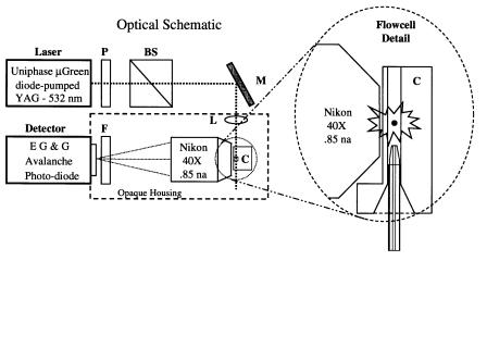
As shown in Figure 6.3, the apparatus is straightforward and uncomplicated. It occupies about 2 ft2 on an optical breadboard. Standard optical mounts are used to hold the various optical components, the laser, and the flow cell. Ancillary items such as two +5-V power supplies, the pressurized sample holder, a compressed nitrogen bottle and pressure regulator, and a data acquisition computer are located nearby.

Laser. The MicroGreen laser (Uniphase, San Jose, CA, www.uniphase.com), a 20mW solid-state, diode-pumped, frequency-doubled neodymium–YAG device, requires neither cooling water nor fans. It is small, produces little heat, runs on 5 V, and has a satisfactory TEM-00 beam shape. Our unit actually produced 36 mW when new (1994), and it still has about 15 mW of output power.

Materials and Methods

121

Fig. 6.3. Optical schematic of the apparatus. The laser output beam passes through a half-wave plate (P) and polarizing beam splitter (BS), which serve to attenuate the laser output power. A mirror (M) and a pair of crossed cylindrical lenses (L) direct the laser light into the flow cell. An optical band pass filter (F, 575DF30) restricts the wavelength range of the light that reaches the APD. The quartz capillary is inserted directly into the 250-µm square channel of the flow cell up to within 500 µm of the laser beam, as shown in the enlarged detail. The laser beam path is out of the page in this drawing.

Beam Shaping Optics. Light from the laser passes through a half-wave plate and a polarizing beam splitter (CVI, Albuquerque, NM; www.cvilaser.com). These two components used together permit continuous adjustment of the laser light intensity that reaches the flow cell. The birefringent element rotates the polarization of the output beam, and the beam splitter dumps the unaccepted light out through one face. The light that passes through the beam splitter is horizontally polarized. For most experiments, only 2–10 mW of laser light is used (measured prior to the mirror). The light that passes through the beam splitter is shaped into an elliptical spot, 11 µm high by 50 µm wide at the sample stream, by a pair of crossed cylindrical lenses of fused silica (Karl Lambrecht, Chicago, IL; www.klccgo.com). A 5-cm-focal-length lens defines the width and a 1-cm-focal-length lens determines the laser beam height. The lenses provide convenient and precise alignment of the laser beam on the sample stream. The laser beam spot size was calculated by the formula

1	4 λ f	(6.1)
spot size =
e2	πD

Where λ = wavelength, f = lens focal length, and D = input beam diameter.

Flow Cell and Fluidics. The laser light is focused on the sample stream inside a custom flow cell (NSG Precision Cells, Farmingdale, NY) with a 250-µm square cross-sectional flow channel, as shown in Figure 6.3. The flow cell is fabricated from several pieces of silica fused together, with one face ground down and polished to the thickness of a microscope cover slip (~70 µm). A modified “Ortho-type” mount

122	Single DNA Fragment Detection by Flow Cytometry

supports the flow cell (with the direction of flow from bottom to top making it easier to eliminate bubbles) and provides the sheath fluid connection and sample entry access. An essential element of the system is a “drain” line at the end of the flow channel that provides back pressure and reduces the flow velocity a thousandfold compared to conventional flow cytometry (FCM). A small piece of soft silastic rubber tubing is pressed gently up to the end of the flow cell, both to create a seal and to connect a 50-cm-length of Teflon tubing (300–400 µm ID) that runs into the bottom of a partially full beaker of wastewater. High-purity water, as sheath fluid, is gravity fed from a 1-l bottle suspended on a post over the instrument. Adjusting both the height of the sheath bottle and the level of the water in the waste container controls the flow velocity. At only 3 ml/h the flow rate is stable over many hours with this simple arrangement. In 1990, Zucker used as much as 150 ft of small-bore tubing to slow the flow in an Ortho instrument (Zucker et al., 1990) and thereby increase its sensitivity. The MiniSizer also slows down the sheath flow by virtue of having the sample delivery capillary inserted directly into, and thereby largely occluding, the flow channel. The small-bore capillary provides high resistance to the sample flow that, combined with the sheath flow restriction, permits stable transit times of 10 ms or more.

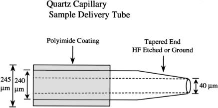
Capillary and Pressurized Sample Delivery. A 30–50-cm-long piece of fused silica capillary tubing (Polymicro Technologies, Phoenix, AZ; www.polymicro.com) delivers the stained DNA molecules directly into the flow cell to within a few hundred micrometers of the laser beam. Capillary tubing of 40 µm ID is normally used, but tubing ranging from 20 to 100 µm ID has been tested. The outer diameter of the capillary, including the polyimide coating that makes it possible to have flexible quartz tubing, is usually about 245 µm. Sheath fluid flows around the capillary in the corners of the 250-µm square cross-sectional flow channel. Perhaps the single most critical item of the entire system is to have a smooth, symmetrical taper on the tip of the capillary (Fig. 6.4). In particular, the rim of the lumen (at the tip) must be as smooth as possible. A rough edge on the tapered end of the capillary invariably resulted in multiple sample streams that caused very confusing behavior of the instrument and usually produced worthless data. However, New Objective (Cambridge, MA; www.newobjective.com) fabricates capillaries for electrospray instrumentation with perfectly tapered ends that are smooth and symmetrical. The desired end result is to have stable, tight, hydrodynamic focusing of the sample stream with the end of the capillary 200–500 µm below the laser beam.

The DNA sample solution is driven through the capillary by nitrogen at a pressure ranging from roughly 0.3 to 1.0 psig. A simple pressure regulator is adequate to maintain stable sample delivery because of the high resistance to flow offered by the capillary tubing and the continuous drain line from the flow cell to the waste container. At 10–11 to 10–13 M (fragments) it is possible to regulate the sample flow rate with a conventional air pressure regulator (Fairchild Model 10, 0–2 psi; www.devicecorp.com). A sample of DNA is diluted in 1X TE buffer to an optimal concentration (about 2 × 10–12 M fragments) in a 1.5-ml Eppendorf tube. The tube fits in a plastic mount, sealed by an O-ring, which supports a rubber septum that is compressed around the capillary and the inlet nitrogen line.

Materials and Methods

123

Fig. 6.4. Detail of the quartz capillary. A smoothly tapered tip is essential and the rim of the capillary lumen must also be smooth in order to prevent multiple sample streams. Examining the sample stream and tip of the capillary through a microscope while a sample of DNA is running in the instrument can reveal if there is a single sample stream and if it is tightly focused.

Detector. The detector is a photon-counting, silicon APD assembly (SPCM-AQ- 121, EG & G, Canada, Vaudreuil, Quebec; www.egginc.com). This sophisticated module utilizes a proprietary circuit that actively quenches the diode and thereby enables it to count photons at rates well in excess of 10 MHz. The diode itself, made from extremely pure silicon, is mounted on a thermoelectric cooling element that eliminates the need for the cumbersome liquid cooling system typically required by a photon-counting photomultiplier tube (PMT). These features serve to keep the dark counts very low [<300 counts per second (cps)]. In this apparatus, as in conventional cytometers, the detector is not the limiting element that determines the detection limit. The dark counts of the detector are overwhelmed by background counts from the laser light impinging on the sheath/sample stream and reflected within the flow cell. An APD module with a dark count rating of < 1000 cps is more than adequate for DNA fragment sizing. Unless other considerations set the noise level, it is desirable to have the lowest possible dark counts for small single-molecule detection.

Light Collection Path. The high-numerical-aperture (NA) Nikon microscope objective (40X 0.84 NA, Melville, NY; www.nikonusa.com) is designed for a maximum working distance of 390 µm in air. The lens has a conventional tube length of 160 mm and a cover glass correction collar to compensate for working distance variations. More light could be collected using an immersion lens, but with the current flow cell dimensions there is not much to be gained. With one wall of the flow cell ground down to 70 µm and the sample stream in the center of the 250-µm-square flow channel, the minimum working distance is 195 µm, well within the objective’s range. An opaque housing covers the flow cell, the microscope objective, the second laser-beam-focusing lens, the band pass filter (Model 575DF30, Omega Optical,

124	Single DNA Fragment Detection by Flow Cytometry

Brattleboro, VT; www.omegafilters.com) and the detector end of the APD module. This permits the system to be operated in normal room lighting.

Data Collection System. A primary raw data set consists of the history of the number of photons registered by the APD detector in small time intervals ranging from 25 to 250 µs, depending on the maximum transit time of individual fragments through the laser beam. A multichannel scaler card (MCS-2, Oxford Instruments, Oak Ridge, TN; www.oxfordinstruments.com) collects the count rate history. The card is essentially a high-speed counter with a programmable count interval and 8192 memory locations into which the count rate history is stored. It counts the transistor–transi- tor–logic (TTL) pulses from the APD, stores the number of detected photon pulses that occur in the dwell time interval, repeats this process until the memory is full, and writes the stored information to a disk file. The dwell time interval used depends on the experiment, that is, whether large or small fragments are being analyzed, and the sample flow velocity. A batch file controls the card, running in a DOS window under Windows 95, in an ISA-bus PC. The batch mode allows multiple scans of the card’s memory to be recorded in separate data files, resulting in a discontinuous count rate history. In order to have meaningful statistics, especially if the DNA sample being analyzed has a heterogeneous mix of fragment sizes, several hundred to 1000 of these small raw data files are collected. While each scan is being written to disk, data collection is interrupted (usually for less than 0.5 s), resulting in a segmented record. Since each scan is written to a separate data file, the first data processing step is to concatenate the raw MCS files into a single large file, which then contains the entire, discontinuous count rate history. The final concatenated file is written to disk with a file header, based on the FCS2.0/3.0 file format standard, that contains all the relevant information about the data collection run, the sample ID, instrument configuration (laser power, optical detection filter, etc.), DNA source, and stain.

In the current configuration, the MCS-2 card resides in a 66-MHz 486 PC clone networked to a second PC, with a shared network drive where the raw data files are written. This second computer, a 200-MHz dual Pentium-Pro PC running WinNT 4.0, is used for all the data processing and analysis. As the raw data files arrive, a program written in the high-level language IDL (Interactive Data Language, RSI, Boulder, CO; wwwrsinc.com) performs the necessary operations on the raw count rate history. The program DNASizer concatenates all the raw data files into one large file (for subsequent storage and analysis under interactive user control). It processes the raw data to sift for the burst events, calculate the primary parameters, and create histograms and various displays. The second computer is sufficiently fast that, within a few seconds after the last raw MCS data file is acquired, the concatenated data file is saved, the entire data set has been processed, and the selected oneand twodimensional histograms and other displays are drawn. At this point the raw MCS files are either deleted or simply overwritten.

It is possible to acquire and process the running count rate history of a photoncounting detector by other means (Agronskaia et al., 1998) but we concluded that it was best to retain the full digital data record. The importance of doing so is supported by studies on the emission dynamics of individual molecules such as phycoerythrin

Materials and Methods

125

which have been observed to abruptly photobleach and to rapidly turn on and off (Wu et al., 1996). These features could easily be lost during D to A and A to D conversions.

Data-Processing Software. Each raw data set contains the entire running count rate history of the APD during the data collection period. In the present photoncounting system, there is no discriminator circuitry to recognize discrete events and extract the pulse parameters of height, width, and area. Since the raw data are a digital record of detected photon counts in small time intervals, they must be sifted via software to identify valid events, correct for the background noise level and the detector’s deadtime, and calculate the primary event parameters. When a data file is first opened, the program automatically evaluates the background noise (in regions of the data set without bursts) and then allows the user to adjust the processing threshold and offset, based on the background and the observed event rate. The processing threshold is the level that identifies the bins to be processed, and the offset is the point (above the threshold) at which a burst is defined to begin. If either of these parameters is modified, the routine sifts an entire selected scan, identifies the bursts, calculates the burst area and duration, and displays a dot plot of the area versus duration for that scan. When the value in a bin exceeds the sum of the threshold and the offset, that bin marks the start of a burst; conversely, when the counts in a bin drop below that level, the burst is terminated. A comparison is then made to determine if the burst falls within minimum and maximum burst length criteria set by the user. If the burst is acceptable, the primary parameters—area, height, and duration—are calculated and stored for subsequent use in creating oneand two-dimensional histograms. The burst area is corrected for the background count rate (the mean count rate in the absence of bursts) by subtracting the background level times the burst duration from the burst area. When the user is satisfied with the settings and the results on the selected scan, clicking on the “Process” button of the data processing panel directs the program to process the entire data set.

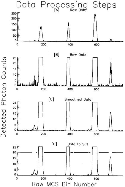
A small section of one raw data set is displayed in Figure 6.5A at a vertical scale that shows the full range of displayed bursts. The second line shows the same data with higher sensitivity (10X vertical gain) to reveal the low-level fluctuations in the count rate history. Many bins in this example recorded zero counts. The first stage of data processing is to smooth the raw count rate history with a fast and efficient smoothing algorithm, built into IDL, known as the Lee filter. This routine calculates local statistics and produces smoothed data that accurately preserve the overall shape and, more importantly, the area of the burst events. It also converts the raw integer data to floating-point numbers with fractional values. The next step is to remove from the data record many of the bins that contain no events and represent only the background count rate of the instrument and sample. In order to minimize coincident events, that is, more than one DNA fragment in the detection volume simultaneously, the DNA sample must be reasonably dilute (6 × 104–6 × 106 fragments/µl) and run slowly (50–250 s–1, depending on the fragment size and flow velocity). Under these conditions, 50–70% of all the bins will contain only background counts. If these bins do not need to be fully processed, eliminating them early in the processing scheme saves considerable time. IDL facilitates such a selection through the use of the

126	Single DNA Fragment Detection by Flow Cytometry

Fig. 6.5. Raw data-processing algorithm. The top line (A) is a segment of the raw data and (B) the same data at a lower y-axis scale to show small fluctuations in the count rate history. (C) Data have been smoothed and converted to floating-point values. Only a small subset of the total raw data—those bins with a count level greater than the processing threshold as drawn in (D)—actually needs to be processed to extract the real events. The horizontal line drawn at the Y value of 20 in (D) indicates the bins that are eliminated when the raw data set is truncated.

Materials and Methods

127

“where” function: “index = where(Raw gt threshold).” This command returns the indices of the bins (in the entire raw data set) where the bin counts are greater than the processing threshold value. One more command, “Raw = Raw(index),” truncates the entire data set, effectively bringing the events closer together than they were in the unedited count rate history. The graph in Figure 6.5D shows the remaining bins that are above the threshold; these are the bins that are sifted in the next processing step to identify and quantify the actual events. This small section of raw data makes a compelling example; of the 800 bins in the original data set, only 200 actually need to be sifted to identify the real events. For the entire data set only 2,614,155 bins out of the initial 4,915,200 required full evaluation. Instead of taking over 50 s to process all of the bins, the routine processed the truncated subset in 28 s. In the data set for Figure 6.1 only 30% of the 2.5 × 106 initial bins had to be sifted. Only the bins retained in the truncated data set receive deadtime correction and final sifting to identify the true events and extract the parametric information from each burst.

A fundamental limitation of the APD detector is that whenever the device detects a photon, it generates a 10-ns-wide TTL pulse and then is unresponsive for an additional 30 ns. However, the manufacturer carefully characterizes the deadtime for each unit (e.g., for one module, the correction factor is 1.25 at 5 mHz and 1.65 at 10 mHz), and it is simple to correct for this limitation, off-line, in software. This is accomplished by correcting the raw count rate history based on the following calculation, which takes into account the bin width (dwell time) of the raw data set and the deadtime of the APD. Because most of IDL’s operators are inherently array oriented, only one line of IDL code [Eq. (6.2)], a straightforward mathematical expression, is required to correct the entire raw data set:

True count rate = Raw ×	1.0		(6.2)
	+ DtFf
	1.0 – (Raw/ b_w) × DeadTime

where Raw is the entire raw data array (the count rate history: 819,200 to 8,192,000 bins), b_w is the programmed dwell time [b_w = float(bin_width) × (1.0 × 10–6)], DeadTime is the specified deadtime for the individual detector, and DtFf is the de- tector-specific fudge factor to better fit the detector’s response curve.

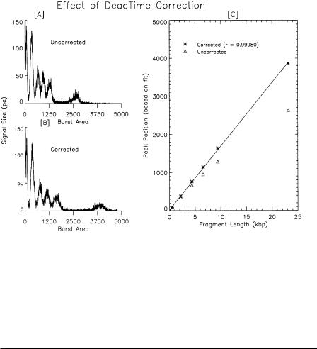
Figure 6.6 (HindIII-digested lambda DNA heated to 60°C for 10 min) graphically reveals the difference between the burst area histograms with and without deadtime correction. Without correction (Fig. 6.6A), the 23-kbp fragment is much closer to the 9.4-kbp peak than it should be. The lower left graph is the histogram produced after the raw count rate history has been corrected. Note that the histogram is not merely shifted to the right. The raw data are corrected on a bin-by-bin basis prior to histogram generation to adjust the measured count rate history to the level expected if the detector did not have a deadtime limitation. In Figure 6.6 the corrected count rate history was resifted and the histogram was recalculated and plotted in panel B. The peak positions plotted in Figure 6.6C are derived from simultaneously fitting six Gaussians to the histograms and then doing linear regression of the known fragment sizes versus the observed signal strength. Space limitations preclude a discussion of the many other analytical features and graphical capabilities of the program.

128	Single DNA Fragment Detection by Flow Cytometry

Fig. 6.6. Effect of deadtime correction. Using the manufacturer’s supplied information on the detectorspecific deadtime, it is possible to correct the raw data for the deadtime of the APD. The upper left-hand panel (A) shows the burst area histogram prior to correcting the raw data and the lower graph (B) is the result of correcting each raw data bin based on the observed count rate, the dwell time, and the deadtime of the APD. On the right is a graph showing the corrected ( ) modal channel values of Gaussians simultaneously fitted to all six peaks in the histogram. Points drawn with triangles are the peak positions prior to deadtime correction.

CRITICAL ASPECTS OF THE SYSTEM

Dye–DNA Interactions

The dye–DNA interactions, which might seem straightforward and uncomplicated, are anything but simple! For POPO-3 (and other related homodimeric, asymmetric cyanine nucleic acid stains), the DNA concentration must be tightly controlled for optimal staining to avoid either DNA precipitation or poorly resolved fragments that would otherwise be resolvable (Rye et al., 1992; Carlsson et al., 1995). Apparently, all of these dyes must be used very carefully and the range of optimal DNA concentrations must be determined experimentally. The bis-intercalating dye molecules have the potential to cross-link separate DNA fragments or to link distant regions on the same fragment, although this seems unlikely (Carlsson et al., 1995). However, the dimer has a very high binding constant compared to the monomers [10–11 vs 10–5 M (Glazer and Rye, 1992; Carlsson et al., 1995)]. As noted earlier, once optimally stained with POPO-3, a sample of DNA (at 450 ng/µl) can be kept at room tempera-