Emerging Tools for Single-Cell Analysis

140	Fluorescence Lifetime Imaging: New Microscopy Technologies

like to move, it is important and useful to know where we are now by considering the historical perspective. In the field of fluorescence, many important experiments were done before the first appearance of the photomultiplier tube in 1948. After being excited to an electronic level, a molecule may follow fluorescence decay. For a single molecular species with one excited electronic state, the decay is an exponential: I(t)=I0exp(–t/τ), where I(t) is the fluorescence intensity at time t, I0 is the fluorescence intensity at t = 0, and τ is the fluorescence lifetime when the intensity reduces to 1/e of the original time-zero intensity. The first measured lifetime value of a fluorescent molecule was determined for fluorescein as 4.5 ± 0.5 ns in 1927 by Gaviola using his first phase-sensitive fluorometer, a sophisticated instrument at the time (Gaviola, 1927). Earlier than that measurement, fluorescence resonance energy transfer (FRET), in which the electronic energy of the excited state of a donor molecule transfers nonradiatively to a receptor, was discovered and demonstrated in 1922 by Cario and Franck (1922). It was later found that energy transfer between molecules depolarized the fluorescence and shortened its lifetime (Gaviola and Pringsheim, 1927). Now FRET is an important tool and has found many applications from studying protein and DNA molecular structure, conformation and kinetics to the organization of membrane structures and drug discoveries (Miki et al., 1998; Visser, 1997; Silverman et al., 1998; Subramaniam et al., 1998; Toth et al., 1998; Clegg, 1996, 1992).

Generally, two methods are utilized to measure the fluorescence decay time, one being the time domain, which includes the time-gating approach, and the other being the frequency domain, or phase modulation method. In the time domain, the fluorescence intensity is recorded as a function of time after a very short pulsed excitation. In the frequency domain, one uses a sinusoidally modulated excitation light source; the phase shift and demodulation of the fluorescence emission are used to calculate the fluorescence decay time. Although in the original fluorescence lifetime measurement the phase modulation method was used, a clever time-domain lifetime measurement without the luxury of fast electronics and detectors was done very early by implementing two electro-optical modulators (Pringsheim, 1949). In this apparatus, the sample was placed between the two Pockels cells in an L-shaped configuration and the detector was placed after the second Pockels cell at the emission side. By varying the distance between the sample and the second Pockels cell for each excitation, the fast fluorescence intensity decay curve can be reconstructed. This type of “time-shifting” method is still used extensively today in both time-domain and fre- quency-domain lifetime imaging systems. After 1950, driven by the needs and interests of biological science, time-resolved spectroscopy developed rapidly using both the frequencyand time-domain method. In the 1980s, the frequency-domain method was significantly refined and automated to be able to measure decays of multiple fluorescent components simultaneously by using multifrequency measurements (Gratton and Limkeman, 1983; Jameson et al, 1984; Gratton et al., 1984).

Overview of Recent Developments in Lifetime Imaging

Currently, fluorescence microscopy and optical microscopy are enjoying a rapid and exciting development period that creates many new possibilities for biomedical research. Since a picture is worth a thousand words, it is the biologist’s dream to be able

Introduction

141

to observe the spatial distribution of relevant signals. Fluorescence time-resolved microscopy imaging is still a relatively new technology. In principle, one may use a normal lifetime spectroscopy instrument by replacing the cuvette sample holder with a microscope and reconstructing a lifetime image point after point (Dix and Verkman, 1990; Keating and Wensel, 1991). This kind of single-point measurement allowed researchers to study specific regions of their samples using a microscope. Certainly, one may choose to spend a large amount of time to obtain a lifetime image this way. To increase the imaging speed, the next development in time-resolved imaging is to use parallel data acquisition with devices such as a charge-coupled device (CCD) camera (Marriott et al., 1991; Wang et al., 1991) or a multianode photomultiplier tube (Morgan et al., 1992). The implementation of laser scanning confocal microscopy, which offers enhanced spatial resolution and enhanced contrast by eliminating out- of-focus emission, increases the sensitivity of lifetime imaging (Piston et al., 1992). Time-resolved fluorescence microscopy using two-photon excitation gives similar confocal spatial resolution with greater background rejection and reduced sample photobleaching (So et al., 1994). In addition, there are many other advantages, such as the reduced effect of photodamage and increased penetration depth of the sample, in using two-photon excitation for imaging living cells (Yu et al., 1996; French et al., 1997) and other vital samples (Masters et al., 1997). Time-resolved microscopy using the time-gated technique (Wang et al., 1991) and phase modulation methods (Marriott et al., 1991; Lakowicz et al., 1992; Piston et al., 1992) dates back to the early 1990s. There are variations of detection techniques used in the frequency-domain fluorescence lifetime imaging. In the case of homodyning detection, where the excitation light source and the detector are modulated at the same frequency, the phase shift and modulation of the fluorescence signal are measured (Clegg et al., 1996; Lakowicz et al., 1992). In the case of heterodyning detection, the detector is gain modulated at a cross-correlation frequency in addition to the modulation frequency for the excitation source. The phase shift and modulation of the signal at the cross-correlation frequency are acquired for calculation of the lifetime value (Mantulin et al., 1993; So et al., 1994). Both homodyning and heterodyning detection methods require a detector with a high-frequency bandwidth in order to measure short-lifetime components. A very interesting variation of the conventional approach is the use of time-correlated optical mixing (Dong et al., 1995, 1997; Buist et al., 1997; Mueller et al., 1995) where two lasers are tuned to different wavelengths, one laser being at the absorption band and the other at the emission band of the fluorescent probe, overlapped in space. The resulting fluorescence signal can be acquired without using fast electronics and detectors. The time-gated method typically uses single-photon counting techniques for the detection and data acquisition, and the phase modulation method mainly uses analog detection and data acquisition schemes. Both techniques have their own advantages and disadvantages that largely depend on the applications and experimental conditions. We will discuss the technical details of both methods later.

Unique Properties of Fluorescence Lifetime

Since the early single-point lifetime microscopy measurements, there have been great technical advances in microscopy and areas of applications using the time-resolved

142	Fluorescence Lifetime Imaging: New Microscopy Technologies

imaging technique. Again, biology plays an important role in enlarging the field of FLIM. Normal biological systems are organized in structurally and functionally unique complexes, which are not homogeneous. Everyone working with fluorescence knows that intensities may vary significantly within the same sample. Often we do not know all the details of the photochemical and photophysical process of the fluorescent probe. It is difficult to quantify what one is interested in measuring with the intensity signal alone. Unlike fluorescence intensity, the lifetime is a fundamental property of a fluorescent molecule, which directly relates to its structure and dynamics. Fluorescence lifetime values typically fall within the range of a few nanoseconds to a few hundred nanoseconds, and the lifetime values of different fluorescent molecules are often different. In some cases the same fluorescent molecule can have very different lifetime values as the probe’s environment changes. For example, ethidium bromide, a nucleotide probe, will have about a 24-ns lifetime when bound to DNA as compared to 1.8 ns when the probe is free in solution (Atherton and Beaumont, 1984). Unlike the intensity measurement, the fluorescent lifetime is not sensitive to the local probe concentration. The lifetime measurement is also much less affected by sample photobleaching. Furthermore, the lifetime measurement provides a different level of discrimination against noise that makes it more immune to scattering and other background noise. An experiment based upon lifetime detection can be very specific as we can choose a probe with distinct and characteristic lifetimes. It can be very sensitive for the signal we are interested in, as we may use the differences in the lifetime to discriminate against autofluorescence, often a significant factor in biological sample. There are also fluorescence probes that are designed specifically for sensing environmental variables such as pH, concentrations of positive and negative ions, viscosity, and oxygen concentration. The inherently high temporal resolution of fluorescence lifetime measurement also allows us to probe rapid dynamics of biological molecules in the time window from microseconds to picoseconds. Integration of the lifetime technique into the conventional confocal microscope and multiphoton microscope will also allow us to have three-dimensional resolution and all the benefits of confocal and multiphoton microscopy. As the lifetime τ of a fluorescent molecule is directly related to its quantum yield ε (τ = ε/κ, κ is the rate constant of the fluorescence decay), lifetime microscopy imaging provides a true quantitative method for conventional microscopy.

FLIM IN THE TIME DOMAIN

Background

It is popular to use time-gated detection in conventional fluorescence lifetime spectroscopy. Several laboratories have developed the lifetime imaging technique using the time-domain approach (Wang et al., 1991; Ni and Melton, 1996; Buurman et al., 1992; Cubeddu et al., 1997; Dowling et al., 1997). There is also a recent report implementing the two-photon scanning technique into the time-domain laser scanning FLIM (Sytsma et al., 1997). The general idea of time-gated detection is to use a short

FLIM in the Time Domain

143

pulse excitation, divide the fluorescence decay curve into several windows of equal time width, record the total fluorescence intensity of each window, and calculate the lifetime. Assuming there is only a single exponential fluorescence decay, the fluorescence signal after a pulse excitation has the form

		τ
F(t) = A exp		– t	(7.1)

where τ is the lifetime, F(t) is the fluorescence intensity at time t after excitation, and A, the preexponential factor, is the zero-time intensity of the fluorescence. The conventional method for cuvette measurement is to acquire many data points along the fluorescence decay curve and to extract the lifetime value τ and the preexponential factor by fitting the data analytically. This approach has been reported in the recent literature using methods similar to the conventional methods used for multiexponential lifetime imaging (Scully et al., 1997; Dowing et al., 1998). This method is difficult to implement in practical real-time imaging with thousands of data points to fit. However, with the help of fast computers and electronics, it is possible to acquire many images along the decay curve and analytically solve multiexponential decays within minutes (Dowing et al., 1998). For FLIM applications, one typically uses the configuration with two time windows (Fig. 7.1), which allows numerical approaches to rapidly determine the lifetime (Woods et al., 1984), and we will discuss this method in more

F i g . 7.1. Time-gating approach for the fluorescence lifetime imaging. T1 and T2 are the beginning time of each time window, F1 and F2 are the total fluorescence intensity collected within the gate width.

144	Fluorescence Lifetime Imaging: New Microscopy Technologies

detail. If δt is the width of the time window, the integrated fluorescence signal within each time window for each pixel (i) within the image follows the equations

	T1				τi
F1,i	= T1	+ δt	Aiexp		– t		dt	(7.2)
	T2				τi
F2,i	= T2	+ δt	Ai exp		– t		dt	(7.3)

Here T2 and T1 are the times at the beginning of each window and F1,i and F2,i are the total intensities within each time window at the i th pixel. The averaged fluorescent

decay time τ can be determined from the ratio of the two integrated intensities (Woods et al., 1984; Ballew and Demas, 1989):

τi	T2 – T1	(7.4)
	=
	ln (F1,i/F2,i)

The preexponential factor can also be calculated as follows:

F1,i

Ai = (7.5)

τi exp(–T1/τi)[1 – exp(–δt/τi)]

The mathematical calculation for the above method is straightforward. Previous work has shown that in the case δt = T2–T1, when the fluorescence signal is optimally used, this rapid lifetime determination method is numerically stable for 0.2δt < τ < 5 δt. To achieve the best sensitivity for a given value of lifetime τ, one should select the gate width or time window to be δt=2.5τ (Ballew and Demas, 1989).

The Instrument

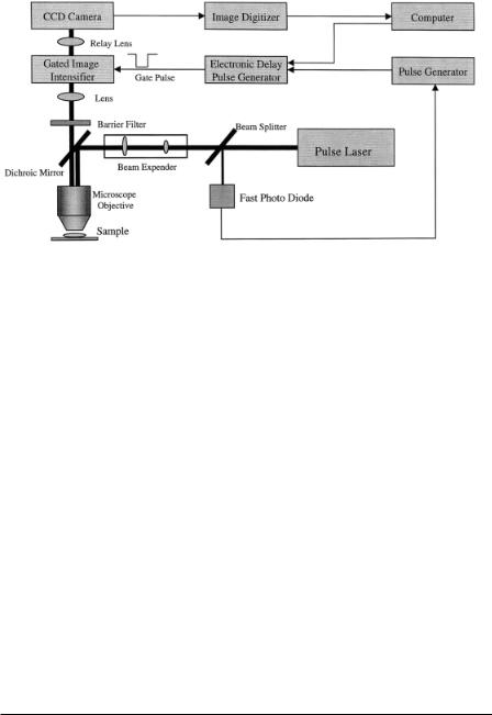
Typical components of a time-gated FLIM apparatus include a microscope, a pulsed laser source, gated image intensifier, CCD camera, image digitizer, and delay pulse generator. A simplified version of a FLIM instrument using the time-domain method is depicted in Figure 7.2. The fast photodiode picks up the oscillation frequency of the laser and divides it into adequate frequency ranges for synchronizing the master pulse generator and the delay pulse generator. The delayed pulse can be controlled through an interface with the computer and is used to gate the image intensifier. The image formed on the phosphor screen is focused onto a CCD camera that can be thermalelectronically cooled to reduce noise. Finally, the gated image, transferred to a computer through an image digitizer, is used for calculating the lifetime.

Pulsed Light Source. A short laser pulse is desirable for the time-gated FLIM method. For the laser pulse repetition rate, it is clear that the higher it is, the faster one may collect sufficient photons. However, higher repetition rates are not always better. For example, the pulse repetition rate of an 80or 76-MHz Ti–sapphire laser is normally too high for most of the fluorescent probes with nanosecond decay times; such high rates can result in incomplete probe recovery for the next excitation pulse and thus complicate data analysis. Pulse pickers, cavity dumpers, and other electro-

FLIM Using Frequency-Domain Homodyning Method

145

F i g . 7.2. Block diagram of a time-gated FLIM instrument.

optical switches are typically implemented to select slower pulse repetition rates in the time-gated detection method. In reality, one finds that the limiting step for selecting the repetition rate is the gating speed of the microchannel plate image intensifier, which is around several tens of kilohertz. In order to efficiently use the photons, one should match the maximum gating speed of the image intensifier with the laser pulse rate. This matching can be done through simple custom-made frequency divider circuitry (Periasamy et al., 1996)

Time Gating of the Detector. The gating mechanism of the microchannel plate image intensifier is achieved by controlling the potential of the photocathode (see Fig. 7.10 later for a drawing of a similar image intensifier). The default potential of the photocathode is set to be positive, which stops the photoelectrons from reaching the microchannel plate, and consequently the image intensifier is in the off state. When a gate pulse arrives at the photocathode with a negative voltage, the image intensifier is switched on and the photoelectrons hit the microchannel plate surface and are amplified, eventually forming an optical image on the phosphor screen. Typically, the gated pulse is controlled through TTL and the gate pulse width is allowed to vary from a few nanoseconds to a few hundred microseconds. Gate widths down to about 100 ps are also commercially available and have been used in time-domain FLIM (Dowling et al., 1998).

FLIM USING FREQUENCY-DOMAIN HOMODYNING METHOD

Background of Frequency-Domain Method

The theoretical background of phase-resolved fluorometry had been given in detail early in the 1930s by Dushinsky (1933), and one can also find details in recent reviews (Clegg and Schneider, 1996). In the frequency-domain method, the fluores-

146	Fluorescence Lifetime Imaging: New Microscopy Technologies

cence sample is excited by an intensity-modulated excitation light source, and typically the modulation is sinusoidal. Under this condition, the fluorescence emission is forced to be sinusoidal, but with a phase delay with respect to the excitation source due to the finite fluorescence decay time. If we assume that the excitation source is modulated at an angular frequency ω, we can describe the fluorescence emission as

F(t) = DC0 + AC0 cos(ωt – φ)

(7.6)

where F(t) is the fluorescence intensity, φ is the phase delay, and DC0 and AC0 are the amplitude of the dc and ac components, respectively. Mathematically, Equation (7.6) is equivalent with Equation (7.1) after Fourier transformation into the frequency space. The ac amplitude of the emission is typically reduced compared to the excitation, a process called amplitude demodulation. Both the phase shift φ and the modulation factor m are functions of the modulation frequency ω. One may use both phase and modulation information to calculate the fluorescence decay time. This scenario of the frequency-domain method is illustrated in Figure 7.3. The lifetime τ, modulation frequency ω, phase shift φ, and modulation factor m preserve the following relationships in a single-exponential case:

φ = arctan (ωφ)	(7.7)
m = 1 2	(7.8)
1 + (ωφ)

The Fourier spectrum (Fig. 7.4) of a single-exponential decay graphically illustrates the relationship among the phase shift φ, the modulation factor m, and the frequency ω. When the modulation frequency ω = 1/τ, the fluorescence has a 45° phase shift, and this phase shift progressively approaches 90° with complete demodulation of the fluorescence signal as the modulation frequency is increased.

The above equations are derived under the assumption that the fluorescence decay is from a homogeneous sample with monoexponential decay constants. However, one can still use them to evaluate multiexponential and nonexponential fluorescence

decay. If τphase is the lifetime calculated from the phase delay and τmod is from the modulation, in the case of a simple single-exponential decay, τphase = τmod. Indeed, if we

measure both τphase and τmod in our experiment, we should be able to tell whether or not we have a single-exponential decay. If the fluorescence is either from a heterogeneous

sample with multiple fluorescence sources each having a different decay constant or from a single fluorescent molecule with multiple decay constants, the calculated life-

times τphase and τmod using Equations (7.7) and (7.8) are no longer the same, and each of them represents the apparent lifetime of the system. If we are in a situation where the

decay is multiexponential, the following relationship holds: τphase < τmod. In the case of a nonexponential decay with a positive preexponential factor, the situation is the same, where the modulation lifetime τmod weights the long-lifetime components and

τphase weights the short lifetime components. The averaged lifetime τaverage of a multicomponent system, as weighted by the intensity fraction f, will not be smaller than

FLIM Using Frequency-Domain Homodyning Method

147

F i g . 7.3. Principle of the frequency-domain approach. Ex(t) is the sinusoidally modulated excitation function with its DCex and ACex components, Em(t) is the corresponding emission function with its own DCem and ACem amplitudies plus a phase shift φ in respect to the excitation. The m is t he modulation factor of the fluorescence signal.

F i g . 7.4. Frequency response of the modulation and phase lag. When the angular modulation frequency ω = 1/τ, then φ = 45°. For a given value of τ, increasing the modulation frequency increases the phase lag and decreases the modulation. To measure a lifetime, one may use modulation frequency ω so that log(ωτ) is within –1 to 1 (shaded area). The best frequency range is when log(ωτ) is between –0.5 to 0.5.

148	Fluorescence Lifetime Imaging: New Microscopy Technologies

τphase in any case. However, the relationship between τmod and τaverage changes following the change of the modulation frequency. Using the equations provided in previous re-

views (Clegg and Schneider, 1996; Jameson et al., 1984), the relationship among

τphase, τmod, τaverage, f, and ω for a system with two-exponential decay, 2 and 20 ns, is graphically represented in Figures 7.5 and 7.6. With the given values of the fractional

contribution of the two individual components, it is seen that both the apparent τphase and τmod progressively decrease with τphase approaching the value of the lower lifetime component as the modulation frequency increases (Fig. 7.5), while τaverage remains stationary. With a given modulation frequency, both τphase and τmod are a function of the fractional contribution. However, at high modulation frequency, τphase is less dependent

on the fraction and stays in the vicinity of the lower lifetime value of the two components up to a sharp turning point.

In the frequency-domain homodyning case, the excitation light source and the fluorescence detector are modulated at the same frequency. In order to measure fluorescence lifetimes in the nanosecond range, the modulation frequency for the light source should be on the order of 10–100 MHz. To directly measure the phase shift and demodulation factor at these frequencies, one requires a digitizer or similar data acquisition device sampling at high speed. Although there are commercially available digitizers working at megahertz and even gigahertz speed, in practice one chooses a different approach for lifetime imaging. Most of the research groups working with homodyning FLIM use the gain-modulated microchannel plate image intensifier and a variable-delay line that controls the phase shift of the modulation

F i g . 7.5. Plot of the apparent lifetime of a system with two equally populated exponential decay (2 ns and 20 ns) components as functions of the modulation frequency ω.

FLIM Using Frequency-Domain Homodyning Method

149

F i g . 7.6. Plot of the apparent lifetimes as functions of the fractional contribution of a system with two exponential decays (2 ns and 20 ns) at a given modulation frequency of A: 10 MHz; B: 40 MHz.

applied on the image intensifier (Hartmann et al., 1997; Mizeret et al., 1997; Clegg et al., 1996; Lakowicz et al., 1994a; Morgan et al., 1992). Using the phase shift of the image intensifier is the key that allows the fluorescence signal at the high modulation frequency to be recorded as steady-state images. Therefore, a slow-scan CCD camera or any digital camera can be used to record the phase-resolved images. One may achieve high accuracy of measurement and phase sensitivity by integrating each image for a length of time without sacrificing any temporal resolution for lifetime imaging.

By using this phase shift method, in principle one may acquire any arbitrary number of images at any different phase values between the detector and the excitation