Emerging Tools for Single-Cell Analysis

160	Fluorescence Lifetime Imaging: New Microscopy Technologies

Fast detectors and associated fast electronics are eliminated using this pump–probe approach. Since short laser pulses contain high harmonics up to hundreds of gigahertz, this method has an extended frequency bandwidth that is not limited by the speed of the detector. The only limiting factor for achieving high temporal resolution using this method is the pulse width of the laser.

Using this pump-probe method, the observable fluorescence signal depends on how well the pump and probe lasers are overlapped in space as well as in time, since the signal can come only from the fluorescent molecules that interact with both lasers. In fact, the nonlinear relationship between the fluorescence intensity and the overlap integral of the intensity of both pump and probe lasers provides high spatial resolution, similar to one-photon confocal and two-photon microscopy in both radial and axial directions (Dong et al., 1997).

The Instrument

Our instrument configuration, shown in Fig7.14, requires two lasers synchronized by a common clock. The detection part of the instrument is simpler than in the normal heterodyning configuration. In particular, the detector does not need to be gain modulated, since the heterodyning occurs in the sample.

Pump and Probe Laser Sources. We use a 10-MHz TTL pulse generated from the master synthesizer (HP8341B, Hewlett Packard) to phase lock both the pump

F i g . 7.13. Principle of the frequency-domain pump-probe method. The first laser beam, oscillating at frequency ω, excites the molecule to the excited states. The second laser beam, oscillating at frequency ω+∆ω, stimulates the molecules back to the ground state. The resulting fluorescence is modulated at frequency ∆ω and its harmonics.

FLIM Using Optical Mixing Methods

161

F i g . 7.14. Instrument diagram of a pump-probe fluorescence microscope for time-resolved imaging in the frequency-domain, deterodyning mode.

laser, an Nd–YAG laser (Antares, Coherent), and the probe laser, a second Nd–YAG laser (Antares, Coherent)–pumped DCM dye laser (Model 700, Coherent). The 532nm laser line of the Nd–YAG laser passing through a second-harmonic generator is used to excite the molecule. The wavelength of the DCM dye laser can be tuned to a wavelength appropriate for the fluorescence emission spectrum of the molecule under investigation. For rhodamine dyes, the DCM laser is typically tuned to around 640 nm. Both Nd–YAG lasers typically operate around 76.2 MHz with a frequency difference of 5 kHz. A combination of Glan-Thompson polarizers can be used to control the laser power and to set the relative polarization between the pump and probe beams. The magic angle condition, which eliminates the polarization effect on the lifetime measurement, can be satisfied conveniently by setting the probe beam 54.7° with respect to the pump beam so that the parallel and perpendicular fluorescence components have a 1:2 ratio going into the detector. Using this setup, the upper limit of the laser power for the pump laser is on the order of microwatts and for the probe beam, it is on the order of milliwatts. The linearity of the signal response to the laser power has been characterized for rhodamine-B in water (Dong et al., 1995). The upper power limit for the pump beam was established at 10 µW and 7 mW for the probe beam for this dye before deviation of the signal.

In addition to the laser arrangement of Figure 7.14, we can also use an alternative configuration in which two Ti–sapphire lasers (Mira 900, Coherent) both pumped by argon-ion lasers (Innova 300, Coherent) are phase locked via a Synchrolock system (model 900, Coherent). In this case, the 80-MHz self-oscillation frequency of one Ti–sapphire laser is used as the clock for locking the second Ti–sapphire laser. The

162	Fluorescence Lifetime Imaging: New Microscopy Technologies

advantage of using the Ti–sapphire lasers is mainly twofold. First, the short pulse width of the Ti–sapphire laser of about 100 fs provides harmonics at hundreds of gigahertz before significant demodulation. Second, the intensity stability of the laser facilitates the measurement and subsequent data analysis. The potential problem with this configuration is the intolerance to any jitter in the phase-locked loop between the two lasers, since the duty cycle of the laser is about 12.5 ns, which is considerably longer than the 100-fs pulse width.

Optics, Signal Detection and Data Acquisition. Both the pump and probe laser beams are collinearly combined on a dichroic mirror before being directed onto the scanning mirrors of the galvanoscanner (model 603X, Cambridge Technology, Watertown, MA). The mirror movement of the scanner is synchronized with the main 10 MHz clock and controlled by the computer. As shown in Figure 7.14, a second dichroic mirror located inside the microscope reflects both laser beams into a highNA microscope objective. The fluorescence signal is collected using the same objective, passed through the same dichroic mirror and 600±20-nm bandpass barrier filters before detection by a PMT (R928 or R1104, Hamamatsu). The signal at the crosscorrelation frequency is first electronically filtered using a preamplifier (Stanford Research, Sunnyvale, CA) and then captured by the data acquisition card for lifetime analysis. As in the case for normal heterodyning using laser scanning, the frame rate depends on the cross-correlation frequency and the number of in-phase averaging. In a typical pump–probe lifetime measurement, the default pixel dwell time is 400 µs, which corresponds to a frame rate of 32 s for a 256 × 256 pixel image.

EXAMPLES OF LIFETIME IMAGING

FLIM is still a relatively new research method not commercially available for many biology laboratories. FLIM research has demonstrated that this new microscopy method is useful for many applications in biological and other systems, including the determination of cellular Ca2+ (Periasamy et al., 1996; So et al., 1995; Piston et al., 1994; Lakowicz et al., 1994a); studying DNA-RNA distribution and local concentrations (Sytsma et al., 1998; Piston et al., 1992); pH variations in different cellular environments (Sanders et al., 1995); membrane fluidity (Yu et al., 1996; Dix and Verkman, 1990); chlorophyll structure and function (Sanders et al., 1996); collagen and elastin autofluorescence (Dowling et al., 1998); tumor detection (Cubeddu et al., 1997; Mizeret et al., 1997; Itoh et al., 1997); oxygen concentration (Hartmann et al., 1997); and thermodynamic studies of combustion (Ni and Melton, 1996). Previously, we have used the capability of our FLIM systems for studying hapten presentation processes in the macrophage (French et al., 1997), membrane fluidity of vital cells (Yu et al., 1996), and cell stress under UVA and near-IR irradiation (Koenig et al., 1996). Important observations have been made in those individual studies because of the lifetime images. Using energy transfer, FLIM has also proven valuable for studying receptor-mediated cellular activities and intracellular vesicle fusion processes (Gadella and Jovin, 1995; Oida et al., 1993).

Examples of Lifetime Imaging

163

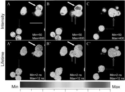
F i g . 7.15. Intensity and lifetime imaging of cellular chloride concentration. The cell is loaded with dihMEQ* and imaged under conditions with 80 MHz and below 4mW laser power at 747 nm using 40x/1.3NA F-Fluar Zeiss objective. The lifetime images are from the modulation measurements. The scale bar is 20 micron. See color plates.

We will now show examples of how using lifetime microscopy imaging is useful in the determination of chloride concentrations within living cells. As a co-factor, chloride regulates cell membrane potential, which is fundamental for cell functions, especially for the cerebral activities (Wagner et al., 1997). Traditionally, chloride concentration is determined by electrophysiological measurement (Krnjevic and Schwartz, 1967). The dynamic quenching by chloride of fluorescence probes such as MEQ, a quinoline derivative, also measures chloride concentrations (Inglefield and Schwartz-Bloom, 1997). However, quenching measurements based solely upon the intensity are not adequate for heterogeneous systems like cells. We will illustrate this point more clearly through the example images.

As a model system, we used the pheochromocytoma cell from rat adrenal gland [PC12 cell, American Type Culture Collection (ATCC), Manassas, VA] cultured in Ham’s F12K medium with 15% horse serum and 2.5% fetal bovine serum. The cell was labeled with the membrane-permeable chloride probe dih-MEQ synthesized from MEQ* (Molecular Probes, Eugene, OR) following the procedures recommended by Molecular Probes. The labeled pc12 cell was washed and suspended in phosphate-buffered saline (PBS) and mounted on a hanging drop microscope slide with a #1.5 glass cover slip.

*MEQ: 6-methoxy-N-ethylquinolinium iodide

164	Fluorescence Lifetime Imaging: New Microscopy Technologies

Examples of the intensity and lifetime image using two-photon scanning FLIM are displayed in Figure 7.15. The intensity images of the cells in panels A, B, and C show high heterogeneity. The areas shown in red color are about 10 times more intense than the areas in dark blue and 3 times more intense than the areas shown in dark green. The lifetime images, on the other hand, show relatively uniform color (panels A′, B′, and C′), which indicates a relative uniform lifetime distributions, partially because the lifetime is fluorophore concentration independent. However, there is still spatial lifetime heterogeneity within these cells. Intensity and lifetime do not have a monotonic relationship. Examples of high intensity correlated with high values of lifetime are indicated by the red arrows in images A, A′ and C, C′. The lifetime value for these red spots is about 12–14 ns, which corresponds to a very low chloride concentration by referencing to the calibration curve (Fig. 7.16) measured in the microscope at the same modulation frequency as that of the cell measurement. This result would imply that the cell accumulates dih-MEQ molecules in a very localized area where the chloride concentration is very low. Examples of high intensity correlated with low lifetime are indicated with white block arrows in images B, B′ and C, C′. The average lifetime value in these regions is about 4.5 ns, which corresponds to 50 mM chloride or more. If we rely only on the intensity data and use intensity quenching as a reference, it would be impossible to correctly interpret the image data in this case. Interestingly, the edge of the cells in the lifetime images show larger than 10 ns lifetime values. This result would be consistent with the exclusion of chloride ion from the plasma membrane. Images A and B are taken in the same field of view but with a few

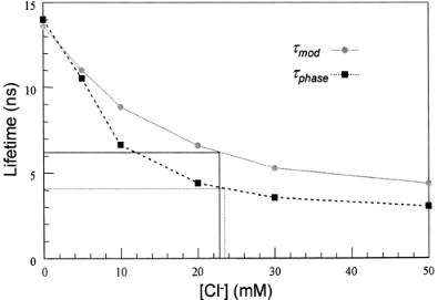
F i g . 7.16. Calibration curve of chloride concentration in deionized water using τmod and τphase. The measurement was performed in the microscope using the 80 MHz modulation frequency at 747nm with a 100-fs

Ti-sapphire laser. The apparent lifetime value is low under this condition and is valid only for calibration of measurements at this modulation frequency.

Examples of Lifetime Imaging

165

F i g . 7.17. Lifetime image of cellular chloride concentration from the phase measurement. The above

image displays τphase value of the same measurement shown in Fig. 7.16B′. Very low lifetime features are indicated by white arrows. The lifetime value for these spots is between 2.0–2.5 ns, which is likely due to

NADH (NAD+) autofluorescence in the mitochondria. The fact that τphase measures the low lifetime components is illustrated in Fig. 7.6B, where the phase lifetime stays low at high modulation even with less

than 30% of total intensity for the component with lower lifetime value. See color plates.

micrometers differences in the focal plane. The cell indicated by the solid white arrows in images A, A′ and B, B′ has a lifetime gradient. This effect is most clearly shown in image B′, where the right side of the cell is blue with average lifetime about 4.5 ns and the left side is more yellow-green with a 5.7-ns average lifetime. In image A′ the same cell is “blue” with about 4.5 ns on average. This result suggests the existence of a chloride gradient from about 30 to 50 mM within a single cell under our experimental conditions.

We have discussed the properties of τmod and τphase in a multicomponent system when using the frequency-domain method. Indeed, the phase lifetime image (Fig. 7.17) shows features of a low lifetime value that are not clearly visible from the

166	Fluorescence Lifetime Imaging: New Microscopy Technologies

modulation lifetime (Fig. 7.15A′) and certainly are not visible from the intensity image (Fig. 7.15A). The averaged lifetime value for the cellular chloride measure-

ment over five to six images gives τmod = 6.25 ns and τphase = 4.0 ns, both falling into an average of about 23 mM of chloride according to our calibration. The fact that

τmod ≠ τphase, indicates a heterogeneous lifetime distribution within individual pixels.

COMPARISON OF DIFFERENT FLIM TECHNIQUES

In some sense, all the FLIM techniques introduced above are unique. The characteristics of the method, such as the sensitivity, photon economy, data acquisition speed, signal-to-noise ratio, and time required for one measurement, very much depend on how the instrument performs and how one does the measurement. There are many variables. It is rather a complicated mathematical task to make a comparison of all the differences. We will point out only some of the major differences, advantages, and shortcomings. To a large extent, some of the shortcomings of a particular method can be overcome by new technological development.

Lifetime Resolution

In the time domain, using the normal two-gated-window method, the width of the excitation pulse and the minimum gate width of the time-gating windows determine the lifetime resolution of the method. This is easy to understand from Figure 7.1, as one can measure the fluorescence only after the decay of the excitation pulse and within the decay time of the fluorescence. If one uses the fastest laser available, the shortest lifetime one may achieve is then limited by the speed of the electronics. It is still possible to measure picosecond lifetimes by using nanosecond gated windows. However, in this case the second gated window will not see much light, and one expects extensive integration will be necessary to collect enough photons. In the case of the frequency domain, using the single-frequency method, the applied modulation frequency to either the excitation source or the detector determines the sensitivity of this method. When a short pulse laser, such as a picosecond or femtosecond laser, is used, the modulation frequency bandwidth of the detector determines the lifetime resolution. Using a typical PMT (R928, Hamamatsu), which can be gain modulated up to 500 MHz–1 GHz (ISS, Champaign, IL), the measurable fluorescence lifetime limit is in the hundred-picosecond range. Certainly, a faster detector such as a modified microchannel plate, which can be modulated up to 10 GHZ, will facilitate measurement of shorter lifetimes.

Photon and Time Efficiency

In the time domain, when the signal from two time-gated windows is collected sequentially after each excitation pulse, the photon and time efficiency is high. It is possible to reach close to 100% efficiency using the emitted fluorescent light (Sytsma et al., 1998) after each pulse. However, in the sequential collection mode, the signal

Comparison of Different Flim Techniques

167

from the two gates cannot be imaged with a single CCD camera. If the signal from the two gates is recorded in two separate passes, the photon efficiency will decrease to one half of that in the previous case. One expects even lower photon efficiency when more than two gates are used. In the frequency domain, when the excitation source and the detectors are sinusoidally modulated, half the fluorescence emission is suppressed. When using the frequency-domain homodyning or heterodyning method, the best photon efficiency is about 50%. However, the amount of fluorescence photons generated strongly depends on the nature of excitation. In the case of pulsed excitation, the number of generated fluorescence photons depends on the frequency of the excitation. In the case of sinusoidally modulated excitation, the photon number depends upon the fluorescence lifetime of the molecule. Indeed, using sinusoidally modulated excitation, more photons are available in the same period of time than with many other means of excitation. Additionally, in the time domain there is a restriction of the highest pulse repetition rate one can use so that there is no second excitation before completion of the previous fluorescence decay.

To decide which method, time domain or frequency domain, is appropriate for a specific application, one should also consider the different detection methods, that is, the single-photon counting or the analog methods. Photon-counting detection has higher photon sensitivity but is susceptible to saturation as compared to the analog detection method. In general, the choice between the time domain and frequency domain depends largely on the fluorescence intensity level of the specimen under investigation. For bright samples the choice is the analog detection and for dim samples the choice is the photon-counting method.

Laser Scanning Versus Wide-Field Illumination

Wide-field illumination is the most common method used in both time-domain and frequency-domain FLIM. With the wide-field illumination one needs an intensified camera either time gated or gain modulated. The cost of such a camera is high. Laser scanning provides an alternative illumination method requiring only single-point detection. The system using a scanner is considerably more cost effective and can be used in both the time-domain FLIM (Sytsma et al., 1998) and the frequency-domain FLIM (Dong et al., 1995; So et al., 1995). The performance and characteristics of the instrument depend on which illumination source is used. Laser scanning using either a two-photon or confocal microscope directly provides three-dimensional sectioned images. The major difference between the two illumination methods is at the detector. Both methods (laser scanning and wide-field illumination) have their advantages and shortcomings and we compare the two cases in the following:

1.Due to the single-point nature of laser scanning, the method is usually associated with single-point detectors such as a PMT. For wide-field illumination, two-dimensional array detectors are typically used. An important advantage of laser scanning is that it allows for imaging regions of interest with arbitrary shapes and for single-point measurements as a function of time. These imaging modes are very useful in biological studies, especially in studies of physiolog-

168	Fluorescence Lifetime Imaging: New Microscopy Technologies

ical functions of live samples. On the other hand, two-dimensional array detectors typically allow imaging of one particular shape depending on the physical arrangement of the detector arrays. The drawback of using scanning is the slower frame rate as compared to that of the array detectors. For fluorescence lifetime imaging, one may reach pixel rates of about 5–10 µs at best using a scanner. With this scanning rate, for a 256 × 256-pixel frame, a frame rate about 0.3–0.6 s is expected, significantly slower than for using normal two-dimen- sional array detectors.

2.For a particular measurement, the laser power per pixel one needs to use is related to the photon sensitivity of the detector and how long one has to integrate for good photon statistics. A camera-based detector made for FLIM applications has an image intensifier that has the same photon sensitivity as a photomultiplier. For a typical image, there are about 105–106 pixels. Using the same laser, the average laser power is about 105–106 times less for wide-field illumination than for laser scanning. To detect the same amount of fluorescence per pixel, the camera has to integrate longer in the case of wide-field illumination as compared to the sequential single-point scanning. However, the total amount of laser energy used for a measurement in the imaging area is about the same.

3.One can use the FLIM method to measure slow decay fluorescence and phosphorescence. In this situation, when using laser scanning, the pixel rate is determined by the decay rate of the fluorophore, allowing sufficient time for the excited molecule to relax to the ground state, as well as collecting enough photons for an accurate lifetime calculation. For instance, if a probe’s lifetime is 1 ms, the required minimum pixel dwell time is approximately 0.01 s and the resulting frame rate for a 256 × 256 pixel image will be on the order of 10 min. Certainly, that would be impractical. For measuring long-lifetime probes, one still needs to integrate over a sufficiently long period for good photon statistics; the practical approach is to use wide-field illumination and two-dimensional array detectors.

Background Rejection and Noise Immunity

For many FLIM applications, we cannot avoid background noise. This noise may arise from autofluorescence or other fluorescence contaminants as well as from stray and scattered light. The lifetime sensitivity of any FLIM method depends on how well the instrument can reject the background noise. To discuss the noise problem, we need to separate the noise that is fluorescent in nature from nonfluorescence noise. For nonfluorescence noise, the frequency-domain heterodyning method provides several noise-suppressing filters, especially the in-phase folding averaging filter, which we believe is superior to other methods. The homodyning method provides a fast Fourier transform and averaging filters for noise suppression. However, by shifting the relative phase between detector and excitation, homodyning measures the dc signal that is subject to interference from very-low-frequency noise. The only filter used

Comparison of Different Flim Techniques

169

in the time-domain method is time-correlated averaging, which is also susceptible to low-frequency noise.

For noise having a decay time, the background varies when using different methods, either the time domain or the frequency domain. In the time domain, the noise is an additional value to the overall intensity. For time-resolved spectroscopy, in the time domain, simple subtraction is sufficient to remove the noise. The scattering noise (τ=0) does not interfere with the measurement. In the frequency domain, the noise, whether the source is fluorescence or scattering, appears as an additional component with its own phase value and modulation amplitude. It is still possible, though complicated, to make background corrections (Reinhart et al., 1991; Swift and Mitchell, 1991; Lakowicz et al., 1987). In principle, the same background correction approach can be used for the FLIM measurement with knowledge of the fractional contribution of the noise for every pixel.

Another issue related to the background correction is to use FLIM to enhance or suppress the contrast of certain lifetime components while not obtaining the lifetime value per se. In this respect, the homodyning FLIM offers a unique mechanism for changing the intensity contrast of a particular lifetime component. This is easy to understand by using Equation (7.16). In the case of homodyning ∆ω = 0,

CC(∆θ) = DC0DCC	AC AC	(7.18)
	+ 0 C cos(∆θ – φ)
	2

and CC(∆θ) becomes a dc value. When the phase difference between the detector and the excitation is set at ∆θ = φ, the cosine has its maximum value and one obtains the maximum intensity contrast for the lifetime component that has phase delay φ at the particular modulation frequency. Similarly, when ∆θ = φ − π/2, the intensity of the lifetime component with delay φ will be suppressed.

Effects of Photobleaching

For FLIM applications, photobleaching normally does not affect the measurement. This is especially true for the time-domain method since the gated channel records only a correlated signal following the fluorescence decay curve. In the frequency domain (homodyning and heterodyning), because the signal is recorded at a lower frequency with respect to the modulation frequency, a steadily decreasing signal could bias the fast Fourier transform, resulting in distortion of phase and modulation values. Photobleaching affects the lifetime measurement at a different time scale for the homodyning and the heterodyning method. In principle, for heterodyning, the measured phase and modulation of the signal will be biased if significant photobleaching happened within the applied cross-correlation frequency, typically on the order of kilohertz for a scanning system. For homodyning, the effect of photobleaching depends on the time factor to acquire the series of images for a single waveform, typically on the order of a second. This photobleaching problem can be addressed by acquiring more data points per waveform not in sequence for homodyning and/or per-