20		1.1.5 Adiabatic equations	[Ref. p. 40
	dJ	= (g(J ) − α) J ,	(1.1.65)
	dz

where g(J ) is the saturated gain coe cient of (1.1.58a), (1.1.58b). For a homogeneously broadened transition and without losses (α = 0) this equation can be can be integrated and provides a transcendental relation for the gain factor G:

G0	= exp	J (0)		f (ω) (G − 1)	(1.1.66)
G		Js

with G0 the small-signal gain factor of (1.1.62) and G the ratio of output/input intensities

G = J (z)/J (0) .

For inhomogeneously broadened transitions a more complicated relation is obtained [81Ver].

*

				- -6

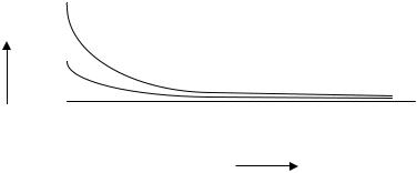
Fig. 1.1.7. Saturation of the gain factor G for a homogeneously and inhomogeneously broadened transition. 1: G0 = 1, 2: G0 = 4, 3: G0 = 6.

1.1.5 Adiabatic equations

If the polarization is in equilibrium with the applied field, without transient oscillations of the electronic system, the interaction is called adiabatic.

1.1.5.1 Rate equations

The field is replaced by the intensity, most spectral e ects are neglected and the rate equations are obtained. They represent an energy balance.

T2 is the time constant, which characterizes the transient behavior of the polarization. In most cases (see Table 1.1.6) T2 is much smaller than T1, and the transient oscillations of the electrons can be neglected. In (1.1.48a) the polarization is replaced by its steady-state value (1.1.50)/(1.1.51) and the rate equations are obtained. They have to be completed by the time-dependent pump term, here labeled as ∆ n0. It depends on the specific pump scheme (see Sect. 1.1.5.3). The rate equations are widely used in laser design to evaluate output power, spiking behavior and Q-switching dynamics. The spontaneous emission contributes to the intensity of the interacting field, but only with a very

Landolt-B¨ornstein

New Series VIII/1A1

Ref. p. 40]	1.1 Fundamentals of the semiclassical laser theory	21

small amount and is neglected here. Nevertheless it is important, because the laser is started by spontaneous emission and in the lower limit it determines the laser band width (Chap. 5.1).

With these approximations the field equations (1.1.48a)/(1.1.48b)/(1.1.48c) for the interaction with a monochromatic field reduce to one equation for the inversion density and a transport equation for the intensity:

∂∆n	=	−	J f (ω)	∆n	−	(∆n − ∆n0)	,	(1.1.67)
∂t			JsT1			T1

∂	+	1 ∂					J = (∆n σ0f (ω)) J	(1.1.68)
∂z			c ∂t

(rate equations for a homogeneously broadened two-level system and a plane monochromatic wave)

with

J (z, t): local intensity,

Js: saturation intensity, depends on the level system (2,3, or 4 levels), see Sects. 1.1.4.1/1.1.5.3, ∆n(z, t): local inversion density.

1.1.5.2 Thermodynamic considerations

So far the interaction with a monochromatic field of intensity J (ω) was discussed. Now the intensity is replaced by the spectral energy density ρω of black-body radiation, providing the Einstein coe cients of spontaneous and induced emission.

Einstein published in 1917 [17Ein] his famous work on the quantum theory of radiation, where for the first time induced emission was introduced, the cornerstone of laser physics. He discussed the two-level system in equilibrium with thermal radiation of spectral energy density ρω (energy per volume and spectral range d ω). The density is given by Planck’s law [61Mor]:

ρω =	ω3	1		VAs2			(1.1.69)
	π2c3		exp [ ω/κT ] − 1		m3

with

κ = 1.38 × 10−23 VAs/K: Boltzmann’s constant.

In thermal equilibrium the levels |ϕ1 , |ϕ2 are populated according to Boltzmann’s law [61Mor]:

n2	= exp [− ωA/κT ] .	(1.1.70)
n1

These two fundamental laws can only be fulfilled, if induced emission is introduced, and Einstein postulated the following equation in steady state for the interaction of thermal radiation with a two-level system:

B12 ρω n1 = B21 ρω n2

+ A21 n2

(1.1.71)

(absorption = induced emission + spontaneous emission)

with

B12, B21, A21: Einstein coe cients of induced and spontaneous emission.

The transition of atoms from the lower level to the upper level by absorption of radiation must be balanced by induced emission and spontaneous emission from the upper level. This equation was

Landolt-B¨ornstein

New Series VIII/1A1