124	3.1.7 Beam propagation in optical systems	[Ref. p. 131

Srotated cyl.

with
A =		0 1
		1 0

and

= R−1 Scyl R = A B

C D

, B =	0 0	, C =		− cos2 θ/fx	− sin θ cos θ/fx		, D =	1 0
	0 0			− sin θ cos θ/fx	− sin2 θ/fx			0 1

O

− sin θ cos θ/fx

− sin2 θ/fx + 1/qyy

Q−1 =

− cos2 θ/fx + 1/qxx

− sin θ cos θ/fx .

Therefore, the output field

k

cos2 θ

1

sin

θ cos θ

u O (r) = exp −i

−

+

x2 − 2

xy +

2

fx

qxx

fx

− sin2 θ + 1 y2

fx qyy

is a general astigmatic Gaussian beam with a mixing term between the coordinates x and y.

3.1.7.3 Waist transformation

Often, the transfer of the beam waist is required for instance for focusing of laser light. Then, the following algorithms are much more simple than the q-parameter algorithm.

3.1.7.3.1 General system (fundamental mode)

In Table 3.1.20 the waist transformation for a general system is given.

3.1.7.3.2 Thin lens (fundamental mode)

The formulae (3.1.123)–(3.1.126) are further simplified using the focal length f for the thin lens only, see Table 3.1.21.

Remark : Discussion of equation (3.1.127):

The right-hand-side term of (3.1.127) containing z0 represents the modification introduced by the Gaussian beam optics to the thin-lens equation ((3.1.95), t 0) shown in Fig. 3.1.42.

In Fig. 3.1.43 the relation of the Gaussian waist transfer to the thin-lens equation of geometrical optics for di erent influences of di raction is shown.

Main modifications of the geometrical optics:

– No “image distance” is at infinity.

–	For z = f (point P ) the image is at z = f (transfer of the object-side focal plane to the image-side
	focal plane after (3.1.130), not ∞).
–	If a target z -position is given, then two starting z-positions are possible.

Example 3.1.17. Given for Fig. 3.1.42: z = 1179 mm, w0 = 0.22 mm, λ = 1.06 µm; it follows z = 109 mm, w0 = 0.02 mm, θ = 0.96◦ , and z0 = 1.21 mm. The second right-hand term of (3.1.127) translates the Gaussian waist image by 0.16 mm in comparison with the geometrical optical image towards the lens.

Landolt-B¨ornstein

New Series VIII/1A1

Ref. p. 131]	3.1 Linear optics	125

Table 3.1.20. Waist transformation for a general system.

Given

Solution

– ABCD-matrix of the system,

z

=

−

B)(Cz + D)

ACz2

–

waist w0,

C2z0

+ (Cz + D)

0 for

(Az + 2

−2

C = 0 ,

–

wavelength λ , including z0 = π w02/λ ,

Az + B

for

C = 0 ,

–

distance z to the input plane of the system.

−

D

(3.1.123)

Cz + A

z0

z 0

z0’

z0

= z0

=

,

Optical system

Cz + D

C2z02 + (Cz + D)2

w

0

characterized by its

’

w ’

(3.1.124)

0

z

A B

- matrix

w0 =

z

C D

λ 0

,

(3.1.125)

z

z ’

π

Θ0

= π z0 .

(3.1.126)

λ

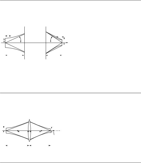
Fig. 3.1.41. Waist transformation by an optical

system.

The beam parameter product is invariant:

Asked : Waist w0 and distance z to the output plane

of the system including z .

= w0 Θ0

= λ/π .

0

w0 Θ0

Table 3.1.21. Waist transformation by a thin lens.

Given

Solution

–

Focal length f of the lens,

1

1

1

2

+

=

+

z0

,

(3.1.127)

–

wavelength λ ,

z [z2 + z02

2

/λ ,

z

z

f

− zf ]

–

waist w0 , including z0 = π w0

see Fig. 3.1.42,

–

distance z to the input plane of the system.

w0 = w0

f

,

(3.1.128)

0

0

z02

+ (z − f )2

w

w ’

π w

2

f

f

z0

=

0

.

(3.1.129)

Image point

λ

of paraxial optics

If z = f , then

z

z ’

z

= f

and

w0 =

w0f

.

(3.1.130)

Fig. 3.1.42. Waist transformation by a thin lens.

z0

Asked : Waist w0 and distance z to the output plane of the system and z0 .

Landolt-B¨ornstein

New Series VIII/1A1