90			3.1.4 Di raction						[Ref. p. 131
x ’						1.0
			x		intensity/	0.8
			x	y			Normalized intensity
	y ’					0.6
a	x				field	0.4		Normalized field
		~ sin
	z				Normalized	0.2
b		z
	Opaque screen			z
						0	FWHM
	Rectangular		Diffraction			0.2
			pattern
	aperture A					0	0.5	1.0	1.5	2.0
								x a/( d )

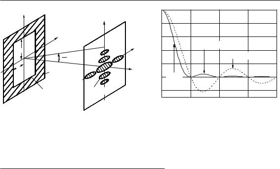
Fig. 3.1.10. Geometry of the di raction from a rectangular aperture 2a × 2b.

Fig. 3.1.11. x-part of the di raction pattern in Fig. 3.1.10. This is the di raction pattern of a slit. For more exact electromagnetic solutions of a slit see [61Hoe, p. 266].

Table 3.1.5. Zeros and maxima of the intensity distribution.

Number n				xa/λz								In/I0
0				0								1
FWHM				2 × 0.221								0.5
1				0.5								0
1				0.715								0.0472
2				1								0
2				1.230								0.0168
3				1.5								0
3				1.735								0.0083
4				2								0
4				2.239								0.0050
Field distribution:
	4 a b			E0 exp −i k z						x2		+ y2		sinc			2 π a x		sinc		2 π b y		(3.1.47)
E(x, y, z) =										+
	i λ z											2 z					λ z				λ z
with sinc(x) =		sin x			and	E0			the electric-field amplitude .
Intensity:				x
										sinc2					.
I(x, y, z) = I(0, 0, z) sinc2							2		λ z					λ z									(3.1.48)
									π a x					2 π b y

If the Fraunhofer di raction is observed in the focal plane, z has to be replaced by f .

3.1.4.4.2 Circular aperture with radius a

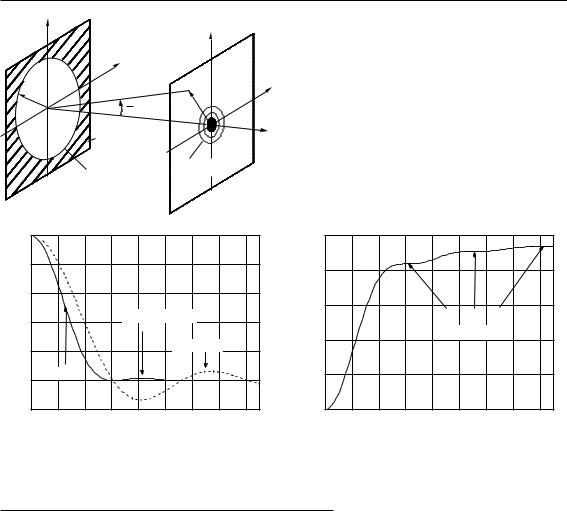
The circular aperture with radius a is discussed in [61Hoe, p. 453]. In Fig. 3.1.12 di raction by a circular aperture is shown. In Fig. 3.1.13a the di racted field and intensity and in Fig. 3.1.13b the encircled energy in the di raction plane with a circular screen are given. The zeros and maxima of intensity for di raction by a circular aperture are listed in Table 3.1.6.

Landolt-B¨ornstein

New Series VIII/1A1

Ref. p. 131]				3.1 Linear optics	91
x			x ’
	y
a	r	~ sin	r	y ’
	d
		d		z
	Opaque screen

						Diffraction
			Circular			pattern
			aperture A
										Fig. 3.1.12. Di raction by a circular aperture.
	1.0										1.0
intensity/fieldNormalized	0.8									encircledNormalizedenergy	0.8
	0.6	FWHM									0.2
				Normalized intensity							0.6				1 st	2 nd		3 rd
	0.4
																dark ring
											0.4
	0.2					Normalized field
	0
0.2											0		0.4		0.8	1.0	1.2		1.4
a	0	0.2	0.4	0.6	0.8	1.0	1.2	1.4	1.6	b	0	0.2		0.6						1.6
					ra/( d )										ra/( d )

Fig. 3.1.13. (a) Di racted field and intensity. (b) Encircled energy in the di raction plane with a circular screen.

Table 3.1.6. Zeros and maxima of intensity for di raction by a circular aperture.

Number n	rna/(λd)	In/I0
0	0	1
FWHM	2 × 0.257	0.5
1	0.610	0
1	0.817	0.0175
2	1.117	0
2	1.340	0.00415
3	1.619	0
3	1.849	0.00160
4	2.121	0
4	2.355	0.00078

Field distribution:
	π a2		−i k	z +	kr2	2	J [2 π a r/(λ z)]
E(r, z) =		E0 exp					1		(3.1.49)
	i λ z				2z		2 π a r/(λ z)

with E0 the electric-field amplitude and r the radius in the far-field plane. Intensity:

I(r) = I(0, z) 2	12 π a r/(λ z)		2	(3.1.50)
			.
	J [2 π a r/(λ z)]

Landolt-B¨ornstein

New Series VIII/1A1