80	3.1.3 Solutions of the wave equation in free space	[Ref. p. 131

3.1.3.2.4.2 Real Bessel beams

Real Bessel beams are limited by a finite aperture D of the optical elements needed or Gaussian beam illumination (Gaussian Bessel beams [87Gor]).

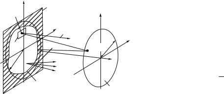
Methods of generation: axicons [85Bic] (Fig. 3.1.2), annular aperture in the focus of a lens [87Dur, 91Nie], holographic [91Lee] or di ractive [96Don] elements. Because of finite aperture di raction the latter display approximately the shape of (3.1.26) with cuto at a geometric determined radius rN , which includes N maxima (Fig. 3.1.3) and di erent amplitude patterns in dependence on z.

B

w

P1

P2 z z 0B

A

Fig. 3.1.2. Generation of a Bessel beam with help of an axicon A by a conus of plane-waves propagation directions.

maximum)
to
(normalized
Intensity	0.2
	0

0	2	4	6	8	10	12
			Radius r

Fig. 3.1.3. Transversal intensity structure of a Bessel beam ( J02(r)).

Advantage of Bessel beams: Large depth of focus 2 z0B between P 1 and P 2 in Fig. 3.1.2 (thin “needle of light”) for measurement purposes.

Disadvantage: Every maximum in Fig. 3.1.3 contains in the corresponding circular ring nearly the same power as the central peak. High power loss occurs if the central part is used only [05Hod].

3.1.3.2.4.3 Vectorial Bessel beams

Vectorial Bessel beams are discussed in [96Hal].

3.1.3.3 Solutions of the slowly varying envelope equation

Gaussian beams are solutions of the SVE-equation (3.1.7) [91Sal, 96Ped, 86Sie, 78Gra], which is equivalent to paraxial approximation or Fresnel’s approximation, see Sect. 3.1.4.

The transition from SVE-approximated Gaussian beams towards an exact solution of the wave equation in the non-paraxial range is given in a Lax-W¨unsche series [75Lax, 79Agr, 92Wue]. For contour plots of the relative errors in the Gaussian beam volume see [97For, 97Zen].

The vectorial field of Gaussian beams is discussed in [79Dav, 95Gou], containing a Lax-W¨unsche series; Gaussian beam in elliptical cylinder coordinates are given in [94Soi, 00Gou].

Landolt-B¨ornstein

New Series VIII/1A1

Ref. p. 131]	3.1 Linear optics	81

3.1.3.3.1 Gauss-Hermite beams (rectangular symmetry)

Elliptical higher-order Gauss-Hermite beam:

Emn(x, y, z) = E0 Um(x, z) Un(y, z) exp {−i k0z} ,

2 Rx(z) exp {i ϕm(z)} ,

(3.1.27)

Um(x, z) = wx(z)

Hm wx(z) exp

− wx2 (z) − i

(3.1.28)

w0x

√

2

x

x2

k0 x2

Un(y, z) = Um n(x y, z)

(3.1.29)

with

w0x : the 1/e2-intensity waist radius,

z0x =

π w02x

: the Rayleigh distance (half depth of focus),

λ

wx(z) = w0x

: the E00-beam 1/e2-intensity radius,

1 + z02

z2

Rx(z) = z 1 +

z2

: the radius of curvature of the wavefront at position z,

z02

1

z

ϕm(z) =

2

+ m arctan

: Gouy’s phase, changing sign for the transition through z = 0,

z0

Hm

√

: the Hermite polynomial of order m [70Abr],

2

wx(z)

H0(ξ) = 1 , H1(ξ) = 2 ξ , H2(ξ) = 4 ξ2 − 2 , H3(ξ) = 8 ξ3 − 12 ξ , H4(ξ) = 16 ξ4 − 48 ξ2 + 12 , . . . ,

∞

exp −ξ2/2

exp −ξ2/2

d ξ

√π m! 2m Hm(ξ)

√π n! 2n Hn(ξ) = δmn ,

−∞

	δmn =	1	for m = n	(orthogonality relation) .
		0	for m = n

Example 3.1.4. Rotational symmetrical Gaussian fundamental mode (Gaussian beam):

Specialization of (3.1.27): m = n = 0 , w0x = w0y = w0 , r =

x2 + y2

.

E00(r, z) = E0

w0

exp −

r2

kr2

exp

i

1

arctan

z

exp {−i kz} ,

− i

w(z)

w2(z)

2R(z)

2

z0

w(z) = w0

, R(z) = z 1 + z02 .

1 + z02

z2

z2

(3.1.30)

(3.1.31)

Properties of E00 (fundamental mode): The shape of the Gaussian E00-beam is depicted in Fig. 3.1.4. Parameters of E00 in Fig. 3.1.4 are:

C : curves with constant amplitude decrease as E(r, z) = E(0, z)/e or constant intensity decrease as I(r, z) = I(0, z)/e2 ,

P : phase fronts with radius of curvature R(z) ,

Landolt-B¨ornstein

New Series VIII/1A1

82	3.1.3 Solutions of the wave equation in free space	[Ref. p. 131

			x
			C			A
	wR		w0	0
			z = 0	P			z
					P	P
		z 0	C			A
				z 0			Fig. 3.1.4. Shape of the Gaussian E00-beam.
	1.0						total	1.0
										P2	P3		P4
r/w)/l(0)	0.8						P(r/w)/P	0.8
	0.6
(							Relativeencircledpower	0.6
Relativeintensityl
			P1							P1
	0.4							0.4
	0.2		P2	P3		P4		0.2
	0							0
		0.5	1.0	1.5	2.0	2.5			0.5	1.0	1.5	2.0	2.5
a	0						b	0
		Relative radial coordinate r /w								Relative radial coordinate r /w

Fig. 3.1.5. (a) Cross section of a Gaussian beam perpendicular to the z-axis. (b) Power transmitted by a circular aperture with the relative radius r/w in a cross section.

Table 3.1.3. Characteristic points in Fig. 3.1.5.

Point in	Relative abscissa	Relative intensity,	Relative transmission,	Characterization
Fig. 3.1.5a, b	r/w	Fig. 3.1.5a	Fig. 3.1.5b
P1	0.588	0.5	0.5	FWHM a
P2	1	0.135	0.865	1/e2-int. b
P3	1.57	0.01	0.99	trunc. c
P4	2.3	0.001	0.999	trunc. d

a Full width half maximum/2.

b 1/e2-intensity or 1/e-amplitude.

c Di raction of E00-beam by circular aperture 17 % intensity ripple [86Sie, p. 667].

dDi raction of E00-beam by circular aperture 1 % intensity ripple [86Sie, p. 667] (no essential e ect of truncation).

w0 : beam waist,

z0 : Rayleigh distance, half of the confocal parameter b = 2z0 (similarly to depth of focus in usual optics), that z-value, where the cross section π wR2 = 2π w02 of the Gaussian beam has doubled in comparison with the waist,

Θ0 = λ/(πw0) : 1/e2-intensity divergence angle toward the asymptotes A.

In Fig. 3.1.5a the cross section of a Gaussian beam perpendicular to the z-axis is given, in Fig. 3.1.5b the power transmitted by a circular aperture with the relative radius r/w in a cross section. Characteristic points in Fig. 3.1.5 are listed in Table 3.1.3.

Astigmatic and general astigmatic generalizations of the elliptical Gaussian beam: see Sect. 3.1.7.

Landolt-B¨ornstein

New Series VIII/1A1

Ref. p. 131]	3.1 Linear optics	83

3.1.3.3.2 Gauss-Laguerre beams (circular symmetry)

√

r

l

2 r2

Elp(r, ψ, z) = E0 exp {−i [kz − ϕlp(z)]}

w0

2

Lpl

w(z)

w(z)

w2(z)

× exp −

r2

k x2

cos (lψ)

− i

sin (lψ)

w2(z)

2 R(z)

with

z : propagation direction,

r, ϕ : polar coordinates in the plane z-axis,

z0 =

πw02

: the Rayleigh distance (half depth of focus),

λ

1 +

z

2

: the E00-beam 1/e2-intensity radius,

w(z) = w0

z0

R(z) = z 1 +

z

2

: the radius of curvature of the wavefront at position z,

0

z

z

ϕlp = (2p + l + 1) arctan : Gouy’s phase, z0

Llp : Laguerre polynomial of degree p and order l [70Abr]:

l

l

l

(l + 1)(l + 2)

− (l + 2) ξ −

1

2

L0

(ξ) = 1 , L1(ξ) = (l + 1)

−

ξ , L2(ξ) =

ξ

,

2

2

l

(ξ) =

(l + 3)(l + 2)(l + 1)

−

(l + 3)(l + 2)

ξ +

(l + 3)

2

1

3

L3

ξ

−

ξ

. . . ,

6

2

2

6

∞

(l + p)!

0

d ξ ξl

exp(−ξ) Lpl (ξ) Lql (ξ) = δpq

(orthogonality relation) ,

p!

p! : the factorial p.

(3.1.32)

(3.1.33)

–Two degenerate mode patterns are formed by the cosand sin-terms in (3.1.32).

–l = p = 0 means the rotational symmetrical Gaussian beam E00.

–The symmetry determines what system of Gauss-Laguerre polynomials or Gauss-Hermite polynomials is more appropriate for a wave field development.

3.1.3.3.3 Cross-sectional shapes of the Gaussian modes

In Fig. 3.1.6 intensity distributions of Gauss-Hermite modes Emn are given (rectangular symmetry), in Fig. 3.1.7 intensity distributions of Gauss-Laguerre modes Epl (circular symmetry).

Landolt-B¨ornstein

New Series VIII/1A1

84		3.1.4 Di raction	[Ref. p. 131
Rectangular symmetry (Gauss-Hermite modes)
00	10	30
y	x
01	11	31

03

13

33

Fig. 3.1.6. Intensity distributions of Gauss-Hermite modes Emn. The two digits at each distribution are m and n.

Circular symmetry (Gauss-Laguerre modes)

00

10

30

01

11

31

03

13

33

Fig. 3.1.7. Intensity distributions of Gauss-Laguerre modes Epl. The two digits at each distribution are p and l. .

3.1.4 Di raction

Di raction of light by aperture rims or amplitude and phase modifications inside the aperture:

–Solutions of Maxwell’s equations taking into account the material properties of the aperture:

–special cases: exact solutions [99Bor, 86Sta],

–mostly: numerical solutions.

–Starting with a field near the aperture with reasonable assumptions for this field or its measurement: large variety of methods for di erent ranges of validity [99Bor, 86Sta, 61Hoe].

Landolt-B¨ornstein

New Series VIII/1A1

Ref. p. 131]	3.1 Linear optics	85

3.1.4.1 Vector theory of di raction

–Vectorial generalization of Kirchho ’s theory: Given E and H in an aperture E and H in the volume by Stratton-Chu Green’s function representation [23Kot, 41Str, 86Sol, 91Ish].

–Two-dimensional problem and meridional incidence of light [61Hoe]: Separation of the polarizations E parallel and E perpendicular to the plane of incidence for half plane [99Bor], slit [99Bor], gratings [80Pet], and volume gratings [69Kog, 81Sol, 81Rus].

3.1.4.2 Scalar di raction theory

Two sources of scalar di raction theory are:

–Transition from vectorial theory to scalar theory: [99Bor, 86Sol]. The information about the polarization is lost.

–Mathematical formulation and generalization of Huygens’ principle: Each point on a wavefront may be regarded as a source of secondary waves, and the position of the wavefront at a later time is determined by the envelope of these secondary waves.

In Table 3.1.4 di raction formulae with fields given near the di raction aperture are listed. Figures 3.1.8 and 3.1.9 are related to Table 3.1.4.

Remarks on the formulae of Table 3.1.4:

(3.1.37): Approximation of (3.1.34): Huygens’ principle with an additional directional factor (Fresnel).

(3.1.38): Approximation of (3.1.36): Huygens’ principle with a modified directional factor.

(3.1.39): Fresnel’s approximation (= paraxial approximation). The approximation conditions from (3.1.34) to (3.1.39) resp. (3.1.40) are explained in [96For, 86Sta, 87Ree].

Fresnel’s approximation: The condition NF(a/d)2/4 1 [91Sal] is valid for sharp-edged apertures A, but it is weakened for the transmission of Gaussian-beam-like fields [86Sie, p. 635] or Gaussian-like soft apertures. Fresnel’s approximation describes the propagation of the field from plane z = 0 to plane z = z. This transformation can be cascaded to describe complex systems and is an often used tool in paraxial propagation of radiation (Sect. 3.1.4.5.2).

	x’	Opaque screen
	S (x’, y’, 0 )
			x
		y ’	Normal
			vector n
	dx ’dy ’	r0	rSP P (x, y, z )
		z = 0
	a		z
			pi
		A

b y

Diffracted field

E (x,y,z)

Fig. 3.1.8. Di raction at an aperture A with source

terms E(x , y , 0) and/or ∂z∂ E(x , y , z) z=0, respectively, and a or b the maximum radial distances

of source S or image point P , respectively. pi symbolizes di erent plane waves for (3.1.41)–(3.1.43).

Landolt-B¨ornstein

New Series VIII/1A1

B¨ornstein-Landolt

VIII/1A1 Series New

Table 3.1.4. Di raction formulae with fields given near the di raction aperture (rSP : see Fig. 3.1.8).

Integrals

Formula

Restrictions

Ref.

Rayleigh-

Sommerfeld of 1st kind

Rayleigh-

Sommerfeld of 2nd kind

Fresnel-Kirchho

RayleighSommerfeld

1st kind approx.

Fresnel-Kirchho approximation, refers to

Fig. 3.1.8

− 4π A

∂ z

rSP

ERS1(x, y, z) =

1

E(x

, y , 0)

∂

exp(−i krSP)

d x d y

ERS2(x, y, z) =

1

A

∂ E(x , y , z

)

z =0

exp(−ikrSP)

d x d y

− 2π

∂ z

rSP

EFK(x, y, z) =

1

[ERS1(x, y, z) + ERS2(x, y, z)]

2

i λ A

rSP

ERS1a(x, y, z) =

1

E(x , y , 0)

exp(−i krSP)

cos (n, rSP) d x d y

i λ A

rSP

·

2

EFKa(x, y, z) =

1

E(x , y , 0)

exp(−i krSP)

1 + cos (n, rSP)

d x

d y

(3.1.34)	rSP > λ0 ,	[99Bor]
	plane aperture	[86Sta]
(3.1.35)	rSP > λ0 ,
	plane aperture
(3.1.36)	rSP > λ0 ,
	curved aperture
(3.1.37)	rSP λ0
(3.1.38)	rSP λ0

Fresnel’s

i exp (−ikz)

A

(x − x )2 + (y

−

y )2

[99Bor]

EFre(x, y, z) =

E(x , y

, 0) exp

i π

d x

d y

(3.1.39) z

λ

[96For]

approximation,

λd

−

λ z

0

[97For]

refers to

[87Ree]

Fig. 3.1.8	[86Sta]
	(continued)

86

ractionDi 4.1.3

131 .p .[Ref

B¨ornstein-Landolt

VIII/1A1 Series New

Table 3.1.4 continued.

Integrals

Formula

Restrictions

Ref.

Fraunhofer

EFra(x, y, z) =

i exp (−i kz) p

A

E(x , y , 0) exp

i 2π

xx + yy

d x

d y

(3.1.40)

a2

1

[99Bor]

far-field

λ z

λd

[68Goo]

λz

approximation,

[96For]

refers to

with the additional phase term

[97For]

Fig. 3.1.8

[86Sta]

p =

b2

1

2

λ z

2

for

λz

1

−

i π x

+ y

otherwise

exp

Plane-wave representation (also: angular-spectrum representation), refers to

Figs. 3.1.8 and 3.1.9

2-D Fourier transform (see remark on (3.1.40)) of the source distribution Es in plane z = 0:

rSP > λ0

[91Sal]

A0(fx, fy ) =

∞ ∞

Es(x , y , 0) exp

i 2 π (fxx

+ fy y

)

d x d y

,

(3.1.41)

[78Loh]

[97For]

[86Sta]

−∞ −∞

[99Bor]

propagation of plane waves with the spatial frequencies fx and fy along the z-direction by distance z:

exp {−i 2 π (fxx + fy y} exp −i 2 π (fxx + fy y +

1/λ2 − fx2 − fy2 z) ,

(3.1.42)

addition of plane waves at distance z:

2

−

E(x, y, z) 2

2

0 x y

x

y

−

x − y

x

y

fx

+fy

<1/λ

A (f , f ) exp

i 2 π

f x + f y +

f 2 f 2 z

d f

d f

,

(3.1.43)

=

1/λ2

equivalent to (3.1.34) [97For]

Far field in the focal plane of a lens, refers to

Fig. 3.1.9

EP(x, y) = λf

∞ ∞

ES(x , y ) exp

i 2 π λf

x

+ λf y dx

dy

,

i p

x

y

−∞ −∞

(x

2

+

y2) (d

f )

p = exp i π

−

λ f 2

d, f λ

[91Sal]

(3.1.44)

(3.1.45)

131] .p .Ref

optics Linear 1.3

87

88			3.1.4 Di raction			[Ref. p. 131
x	Plane wave		x ’	Field ES (x’,y’)	Lens	x
				Plane wave		Convergent wave
						z
	x	= sin	1			Field EP (x,y)
			x
				d		f
x = 1/fx			z
a			b
Fig. 3.1.9. (a) Spatial frequencies of a plane wave with propagation direction Θx with respect to the
plane x = 0 (and Θy analogously) are fx and fy with Θx = sin−1(λfx) ≈ λfx and Θy = sin−1(λfy ) ≈ λfy
(≈: paraxial approximation). (b) Generation of the far field in the focal plane of a lens: The Fourier
transformation (d = f ) is changed by an additional phase term for d = f with d: distance, f : focal length.

(3.1.40): Fraunhofer’s approximation

– Fresnel number :

NF = a2/λz .

(3.1.46)

–Validity of Fraunhofer’s approximation: NF 1 .

p = 1 (parabolic phase): the intensity of di racted light is the square of the modulus of the Fourier transform of E(x, y, 0) only.

– Additional condition with second Fresnel number NF = b2/λz 1 :

E(x, y, z) is the Fourier transform of E(x, y, 0) in dependence on the spatial frequencies fx ≈ (x/z)/λ ≈ Θx/λ and fy ≈ (y/z)/λ ≈ Θy /λ .

– Di erent conventions on the spatial Fourier transform F (fx) of a spatial distribution f (x) :

–The convention of the plane-wave structure exp(i kx − i ω t) is connected with the determination of F (fx) by

∞

F (fx) = d x f (x) e−i 2π fxx

−∞

[68Goo, 68Pap, 78Loh, 78Gas, 93Sto, 05Hod].

– The plane-wave structure exp(i ω t − i kx) can be combined with

∞

F (fx) = d x f (x) ei 2π fxx

−∞

[71Col, 73Men, 92Lug], but

∞

F (fx) = d x f (x) e−i 2π fxx

−∞

is defined also in [88Kle, 91Sal, 95Wil, 96Ped].

Landolt-B¨ornstein

New Series VIII/1A1

Ref. p. 131]	3.1 Linear optics	89

– Di erent approximations in (3.1.37) and (3.1.38):

rSP ≈ r0 + 2xξ − ξ2 + 2yη − η2

2r0

[99Bor, 68Pap, 78Gra] with r0 from Fig. 3.1.8 versus

rSP ≈ z + 2xx − x 2 + 2yy − y 2

2z

(references on lasers: [86Sie, 05Hod], optoelectronics: [68Goo, 72Mar, 91Sal]) for grating di raction: The sine of the di raction angle sin Θx = x/r0 is derived from principle and not by a postpositive reasoning of the paraxial range x/z = tan Θx ≈ sin Θx. x/z should be “translated” into sin Θx for better approximation.

(3.1.41)–(3.1.43): Plane-wave spectrum or angular-spectrum representation (also Rayleigh- Sommerfeld-Debye di raction theory) [78Loh, 99Pau] is the plane-wave formulation of (3.1.34) [78Loh, 97For]. Application: see Fourier optics [68Goo, 83Ste, 93Sto].

(3.1.44), (3.1.45): Generation of the far field in the focal plane of a lens: d = f (object is outside the object-side focal plane) additional phase term p to the pure (inverse) Fourier transform (d = f ), similarly to (3.1.40).

Applications: generation of the spectrum of a function, possibility of mathematical operations in the Fourier-space with complex filtering masks, correlation and convolution.

Another important di raction theory

Di raction theory after Young, Maggi, Rubinowicz [66Rub, 99Pau]: The light in point P of Fig. 3.1.8 results from the unperturbed light and local waves, which are emitted by the edge of the aperture A. Therefore, a line integral is to be calculated [99Pau]. There is an equivalence with Fresnel-Kirchho ’s theory.

3.1.4.3 Time-dependent di raction theory

Two formulations of the time-dependent treatment of di raction are possible:

1.A general Fresnel-Kirchho ’s integral formula exists for time-dependent source functions in the aperture A, see [99Bor, 99Pau].

2.Used more often now [96Die, 99Pau]: The time-dependent source functions are decomposed into a superposition of monochromatic fields. The di racted field is calculated for every monochromatic component by the stationary di raction given above. The superposition of all di racted monochromatic components yields the time-dependent di racted field.

3.1.4.4 Fraunhofer di raction patterns

3.1.4.4.1 Rectangular aperture with dimensions 2a × 2b

In Fig. 3.1.10 the geometry of the di raction from a rectangular aperture 2a × 2b is shown. The x-part of the di raction pattern in Fig. 3.1.10 is given in Fig. 3.1.11. In Table 3.1.5 the zeros and maxima of the intensity distribution are listed.

Landolt-B¨ornstein

New Series VIII/1A1