104		3.1.5 Optical materials	[Ref. p. 131
	x
	Planes of
	constant
	amplitude
	T	z
n	n ’ ik ’
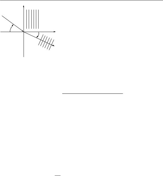
	Planes of	Fig. 3.1.25. Refraction at a medium with absorption: generation
	constant
	phase	of an inhomogeneous wave.

Inhomogeneous wave (Fig. 3.1.25): Snell’s refraction law is modified:

sin ΘT =	n	sin Θ	(3.1.82)
	nT

with

2 n2T = n 2 − k 2 + n2 sin2 Θ + n 2 − k 2 − n2 sin2 Θ 2 + 4 n 2 k 2 (Ketteler’s formula) .

The e ective refractive index nT determines the direction angle ΘT of planes of constant phase in Fig. 3.1.25 via (3.1.82) [88Kle, p. 78], [41Str, p. 503], [99Bor, p. 740]. The full inhomogeneous wave can be calculated using [99Bor, p. 740].

Example 3.1.11. Θ = 45 ◦, Au: λ = 800 nm, n = 0.19, k = 4.9, nT = 0.73, ΘT = 75.1 ◦ (see [28Koe, p. 209]).

Intensity attenuation in the case Θ = 0 ◦:

I = I0 exp {−2

(ω/c) k z} .

−

(3.1.83)

1/e − depth = 13 nm.

◦

, Au: λ = 800 nm, n

= 0.19, k

= 4.9,

I = I

0

exp

×

,

Example 3.1.12. Θ

= 0

7.7

104 z[mm]

p −

s

|rs|

p

|

p|

p

s

|

s|

s

Ellipsometry: δ

δ

and moduli

|rp|

of the reflected light r

=

r

exp (i δ

) and r

=

r

exp (i δ

)

can be measured. The complex refractive index of a material results [77Azz, 90Roe]. Application: Measurements for the optical constants of metals, semiconductors, and thin-film systems.

3.1.5.7 Crystal optics

3.1.5.7.1 Classification

The dielectric tensor εr = εij in (1.1.8) is symmetrical and real in the case of a nonabsorbing medium.

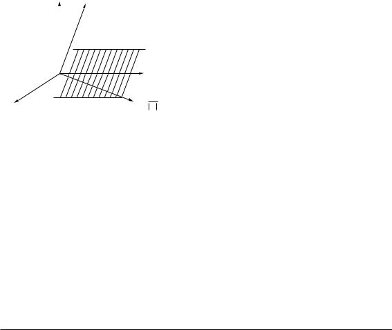
In Fig. 3.1.26 vectors connected with wave propagation in crystal optics are depicted. In Table 3.1.8 optical crystals are listed. In Table 3.1.9 three of the eight surfaces for visualization of wave propagation in crystals are presented.

Landolt-B¨ornstein

New Series VIII/1A1

Ref. p. 131]						3.1 Linear optics		105
E			D
			Beam edge
						Fig. 3.1.26. Vectors connected with wave propagation in
				s		crystal optics [99Bor]: s : ray direction unit vector Poynt-
						ing vector E × H, n : unit vector in the normal direction
B, H			Beam edge	n =	k	k and phase planes, orthogonalities: B, H E, D, n, s ;
					k
						E s ; D n.
Table 3.1.8. Optical crystals.
Classification:			Refractive index			Optical type	Example	Values of the
system (syngony)			in the main axis			of crystal		refractive index
of crystal			system					for λ = 589.3 nm
triclinic,			nx = ny = nz = nx			biaxial crystal, no	NaNO3	nx = 1.344 ,
monoclinic,						ordinary waves		ny = 1.411 ,
orthorhombic								nz = 1.651
trigonal,			nx = ny = no			positive uniaxial	SiO2	no = 1.544,
tetragonal,			(ordinary			crystal: no < ne	(quartz)	ne = 1.553
hexagonal			index)
			nx = nz = ne			negative uniaxial	CaCO3	no = 1.658,
			(extraordinary			crystal: no > ne	(calcite)	ne = 1.486
			index)
cubic			nx = ny = nz = n			isotropic crystal	NaCl	n = 1.544

Table 3.1.9. Three of the eight surfaces for visualization of wave propagation in crystals.

Surface	Given	Found by construction are the
Index ellipsoid (indicatrix)	normal direction n	D-vectors for the two polarization cases
(one-shell surface)		and the two refractive indices for phase
		propagation
Index surface, wave vector	normal direction n ray directions s, which are perpendicular
surface (two-shell surface)		to the surface for both polarization cases
Ray surface, wave surface, representing	ray direction s	normal direction n, which is perpendicular
Huygens’ elementary wave for both		to the surface
polarization cases (two-shell surface)

Main feature of crystal optics: s is not parallel with n for wave propagation, mostly.

–s is essential for description of the energy propagation (edges of bundles, rays),

–n is essential for description of the interferences of infinite broad waves.

References: [28Szi, 54Bel, 58Shu, 61Ram, 76Fed, 79Wah, 84Yar, 04Ber, 99Pau, 99Bor]. A detailed comparison between that surfaces is given in [28Szi].

Landolt-B¨ornstein

New Series VIII/1A1

4B2

n2θ e

= BA +

106	3.1.5 Optical materials	[Ref. p. 131

3.1.5.7.2 Birefringence (example: uniaxial crystals)

Uniaxial crystals in the plane of incidence:

–Refraction of the normal direction n of wavefronts: The wavevector surface is shown in Fig. 3.1.27.

sin Θo =	n	sin Θ (ordinary wave (ko))			(3.1.84)
	no
(no does not depend on the angle of incidence),
		n
sin Θe =			sin Θ	(extraordinary wave (ke))	(3.1.85)
	nθ e (Θe(Θ))

(ne depends on the angle of incidence).

–Refraction of rays (Poynting vector): se and so are given by tangent construction in Fig. 3.1.28.

–Algorithm for the calculation of ko ( so), ke, se of Fig. 3.1.28 with n, no, ne, η, θ of Fig. 3.1.29 [86Haf]:

n2(n2o − n2e )2 sin2 Θ sin2(2η) 2 B2

2

n2)2

sin Θ sin (2η)

× n2 sin2 Θ

(n2

n2)2

sin2(2η)

A

±

n(no

−

e

o

−

e

− 1 +

(3.1.86)

B

B

(refractive index for the extraordinary wave)

with

A = (n2e − n2o) n2 sin2 Θ cos (2η) − n2o n2e ,

B = n2o + (n2e − n2o) sin2 η ,

where the decision on the ± sign in (3.1.86) can be made by controlling the satisfaction of

n2θ e n2o + (n2e − n2o) sin2(η + Θe) = n2e n2o .

The resulting angles are:
Θo = arcsin(n sin Θ/no) ,							(3.1.87)
	x
Optical axis
				TE
		k o			k e	TM
			o e				z
	k
Polarization							Fig. 3.1.27. Construction of wavefront birefringence with
TE and TM
Index n				Indices no and ne			the wavevector surface: The wavefronts show no transversal
							limitation.

Landolt-B¨ornstein

New Series VIII/1A1