38	C. Couprie et al.

most cases is set to be a scalar functional with values in R+. In other words, the GAC equation finds the solution of:

argminC g(s)ds,	(3.5)
C

where C is a closed contour or surface. This is the minimal closed path or minimal closed surface problem, i.e. finding the closed contour (or surface) with minimum weight defined by g. In addition to simplified understanding and improved consistency, (3.4) has the required form for Weickert’s PDE operator splitting [28, 68], allowed PDEs to be solved using separated semi-implicit schemes for improved efficiency. These advances made GAC a reference method for segmentation, which is now widely used and implemented in many software packages such as ITK. The GAC is an important interactive segmentation method due to the importance of initial contour placement, as with all level-sets methods. Constraints such as forbidden or attracting zones can all be set through the control of function g, which has an easy interpretation.

As an example, to attract the GAC towards zones of actual image contours, we could set

g ≡	1	,	(3.6)
	1 + | I|p

With p = 1 or 2. We see that for this function, g is small (costs little) for zones where the gradient is high. Many other functions, monotonically decreasing for increasing values for I, can be used instead. One point to note, is that GAC has a so-called shrinking bias, due to the fact that the globally optimal solution for (3.5) is simply the null contour (the energy is then zero). In practice, this can be avoided with balloon forces but the model is again non-geometric. Because GAC can only find a local optimum, this is not a serious problem, but this does mean that contours are biased towards smaller solutions.

3.2.5 Graph-Based Methods

The solution to (3.5) proposed in the previous section was in fact inspired by preexisting discrete solutions to the same problem. On computers, talking about continuous-form solutions is a bit of a misnomer. Only the mathematical formulation is continuous, the computations and the algorithms are all necessarily discrete to be computable. The idea behind discrete algorithm is to embrace this constraint and embed the discrete nature of numerical images in the formulation itself.

3.2.5.1 Graph Cuts

We consider an image as a graph Γ (V , E ) composed of n vertices V and m edges E . For instance, a 2D N × N 4-connected square grid image will have n = N2 vertices

3 Seeded Segmentation Methods for Medical Image Analysis

39

and m = 2 × N × (N − 1) edges.1 We assume that both the edges and the vertices are weighted. The vertices will typically hold image pixel values and the edge values relate to the gradient between their corresponding adjacent pixels, but this is not necessary. We assume furthermore that a segmentation of the graph can be represented as a graph partition, i.e:

V = Vi; i =j,Vj ∩Vi = 0/.	(3.7)
Vi Γ

Then E is the set of edges that are such that their corresponding vertices are in different partitions.

E = {e = {pi, p j} E, pi Vi; p j Vj, i =j}.

(3.8)

The set E is called the cut, and the cost of the cut is the sum of the edge weights

that belong to the cut:	∑ we,
C(E ) =		(3.9)

e E

where we is the weight of individual edge e. We assume these weights to be positive. Reinterpreting these weights as capacities, and specifying a set of vertices as connected to a source s and a distinct set connected to a sink t, the celebrated 1962 Ford and Fulkerson result [25] is the following:

Theorem 3.1. Let P be a path in Γ from s to t. A flow through that path is a quantity which is constrained by the minimum capacity along the path. The edges with this capacity are said to be saturated, i.e. the flow that goes through them is equal to their capacity. For a finite graph, there exists a maximum flow that can go through the whole graph Γ. This maximum flow saturates a set of edges Es. This set of edges define a cut between s and t, and this cut has minimal weight.

This theorem is illustrated in Fig. 3.2.

In 2D and if Γ is planar, this duality essentially says that the Ford and Fulkerson minimum cut can be interpreted as a shortest path in a suitable dual graph to Γ [2]. In arbitrary dimension, the maxflow – mincut duality allows us to compute discrete minimal hypersurfaces by optimizing a discrete version of (3.4).

There exist many algorithms that can be used to compute the maximum flow in a graph (also called network in this framework), but none with a linear complexity. Augmenting paths algorithms [7] are effective in 2D where the number of vertices is relatively high compared to the number of edges. In 3D and above, where the reverse is true, push-relabel algorithms [27] are more efficient. These algorithms can only be used when there is one source and one sink. The case where there are multiple sources or sinks is known to be NP-hard. To compute energies comprising several sources or sinks and leading to multi-label segmentation, approximations

1This particular computation is left as an exercise to the reader.

40	C. Couprie et al.
a	b
S	S

t

t

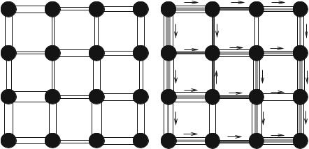
Fig. 3.2 (a) A graph with edge weights interpreted as capacities, shown as varying diameters in this case. (b) A maximum flow on this graph. We see that the saturated vertices (in black) separate s from t, and they form a cut of minimum weight

can be used, such as α -expansions. These can be used to formulate and optimize complex discrete energies with MRF interpretations [8, 66], but the solution is only approximate. Under some conditions, the result is not necessarily a local minimum of the energy, but can be guaranteed not to be too far from the globally optimal energy (within a known factor, often 2).

In the last 10 years, GC methods have become extremely popular due to their ability to solve a large number of problems in computer vision, particularly in stereo-vision and image restoration. In image analysis, their ability to form a globally optimal binary partition with a geometric interpretation is very useful. However, GC do have some drawbacks. They are not easy to parallelize, they are not very efficient in 3D, they have a so-called shrinking bias, just as GAC and continuous maxflow have as well. In addition, they have a grid bias, meaning that they tend to find contours and surfaces that follow the principal directions of the underlying graph. This results in “blocky” artifacts, which may or may not be problematic.

Due to their relationship with sources and sinks, which can be seen as internal and external markers, as well as their ability to modify the weights in the graph to select or exclude zones, GC are at least as interactive as the continuous methods of previous sections.

3.2.5.2 Random Walkers

In order to correct some of the problems inherent to graph cuts, Grady introduced the Random Walker (RW) in 2004 [29,32]. We set ourselves in the same framework as in the Graph Cuts case with a weighted graph, but we consider from the start

3 Seeded Segmentation Methods for Medical Image Analysis

41

a multilabel problem, and, without loss of generality, we assume that the edge weights are all normalized between 0 and 1. This way, they represent the probability that a random particle may cross a particular edge to move from a vertex to a neighboring one. Given a set of starting points on this graph for each label, the algorithm considers the probability for a particle moving freely and randomly on this weighted graph to reach any arbitrary unlabelled vertex in the graph before any other coming from the other labels. A vector of probabilities, one for each label, is therefore computed at each unlabeled vertex. The algorithm considers the computed probabilities at each vertex and assigns the label of the highest probability to that vertex.

Intuitively, if close to a label starting point the edge weights are close to 1, then its corresponding “random walker” will indeed walk around freely, and the probability to encounter it will be high. So the label is likely to spread unless some other labels are nearby. Conversely, if somewhere edge weights are low, then the RW will have trouble crossing these edges. To relate these observations to segmentation, let us assume that edge weights are high within objects and low near edge boundaries. Furthermore, suppose that a label starting point is set within an object of interest while some other labels are set outside of it. In this situation, the RW is likely to assign the same label to the entire object and no further, because it spreads quickly within the object but is essentially stopped a the boundary. Conversely, the RW spreads the other labels outside the object, which are also stopped at the boundary. Eventually, the whole image is labeled with the object of interest consistently labeled with a single value.

This process is similar in some way to classical segmentation procedures like seeded region growing [1], but has some interesting differentiating properties and characteristics. First, even though the RW explanation sounds stochastic, in reality the probability computations are deterministic. Indeed, there is a strong relationship between random walks on discrete graphs and various physical interpretations. For instance, if we equate an edge weight with an electrical resistance with the same value, thereby forming a resistance lattice, and if we set a starting label at 1 V and all the other labels to zero volt, then the probability of the RW to reach a particular vertex will be the same as its voltage calculated by the classical Kirchhoff’s laws on the resistance lattice [24]. The problem of computing these voltages or probability is also the same as solving the discrete Dirichlet problem for the Laplace equation, i.e. the equivalent of solving 2ϕ = 0 in the continuous domain with some suitable boundary conditions [38]. To solve the discrete version of this equation, discrete calculus can be used [33], which in this case boils down to inverting the graph Laplacian matrix. This is not too costly as it is large but very sparse. Typically calculating the RW is less costly and more easily parallelizable than GC, as it exploits the many advances realized in numerical analysis and linear algebra over the past few decades.

The RW method has some interesting properties with respect to segmentation. It is quite robust to noise and can cope well with weak boundaries (see Fig. 3.3). Remarkably, in spite of the RW being a purely discrete process, it exhibits no grid bias. This is due to the fact that level lines of the resistance distance (i.e. the