210	M.A. Haidekker and G. Dougherty

above the inverse spatial distance of the image features of interest, can be omitted from the computation of any frequency-domain metric, leading to an immediate reduction of the influence of noise. Application of a moderate spatial-domain noise filter before performing the Fourier transform is none the less advisable, because it reduces aliasing artifacts.

9.3.4 Use of Fractal Dimension Estimators for Texture Analysis

Fractal models enjoy great popularity for modeling the texture in medical images, with the fractal dimension commonly used as a compact descriptor. The fractal dimension D describes how an object occupies space and is related to the complexity of its structure: it gives a numerical measure of the degree of boundary irregularity or surface roughness. In its original mathematical definition, a fractal object is created by a set of mapping rules that are applied iteratively on an object. After an infinite application of the mapping operation, the resulting object is invariant under the mapping operation and therefore referred to as the attractor of the mapping rules. The attractor is self-similar in the sense that any part, magnified, looks like the whole. Furthermore, the mapping rules determine the self-similarity dimension of the attractor, which is strictly less than, or equal to, the Euclidean dimension E of the embedding space (E = 1 for a line, E = 2 for a surface, and E = 3 for a volume). In nature, self-similarity occurs, but contains a certain degree of randomness. For this reason, no strict self-similarity dimension exists, and the apparent fractal dimension needs to be estimated by suitable methods. To cover the details of this comprehensive topic is beyond the scope of this chapter. A highly detailed overview of the subject with a mathematical focus can be found in [53], the groundbreaking work by Mandelbrot [54] deals with the aspect of randomness in natural fractal objects, and an in-depth overview of the methodology of estimating fractal dimensions in images can be found in [39].

Fractal analysis always involves the detection and quantification of self-similar behavior, i.e., to find a scaling rule under which a magnified part of the image feature is similar to the whole. This property can be illustrated with the example of the coastline of England. The length of the coastline can be estimated with calipers. However, as the caliper setting is reduced, the length of the coastline appears increased, because the caliper now covers more of the smaller detail, such as bays and headlands. In fact, nonlinear regression of the coastline length l as a function of the caliper setting s reveals a power law,

	l =	1	(9.9)
		sD

where D is the apparent fractal dimension. Equation (9.9) implies that the measured length exceeds all bounds as s → 0, which is indeed a property of some mathematical fractals. In actual images, the scaling law fails when the limits of the resolution

9		Medical Imaging in the Diagnosis of Osteoporosis...										211
	a										b

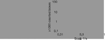
Fig. 9.8 Demonstration of the box-counting method to estimate the fractal dimension of binary images. The image (a) shows the water body (black) of the Amazon river. Superimposed is a square mesh of boxes. Every box that contains or touches the river is counted. Next, the mesh is refined (usually by powers of two), and the number of smaller boxes containing part of the river is counted again. If self-similar properties exist, the log-transformed number of boxes, plotted over the log-transformed inverse box size (b), will follow a straight line with slope D

are reached. In practice, the range of scales under which a scaling law similar to (9.9) can be found is even more limited. In the example of the coastline, values around D = 1.2 can be found [39, 53]. This is consistent with the notion of a very complex and convoluted line embedded in two-dimensional Euclidean space, where 1 ≤ D ≤ 2. A surface, such as a grayscale elevation landscape, is embedded in threedimensional space, where 2 ≤ D ≤ 3 holds.

A very widespread method to estimate an apparent fractal dimension in binary images is the box-counting method, explained in Fig. 9.8. The feature needs to be segmented (the river in the example), and the number of boxes that contain part of the feature are counted as a function of the box size. If a power-law similar to (9.9) exists, the counted boxes NB over the inverse scale 1/s lie on a straight line in a log–log plot, and nonlinear regression yields the box-counting dimension DB:

log NB = −DB · logs

(9.10)

In a grayscale extension of the box-counting method, the image intensities are interpreted as heights in an elevation landscape. The surface area is determined, whereby the scale is controlled by averaging neighboring pixel values inside boxes of a grid. Numerous other algorithms for estimating fractal dimension have been described [39, 55, 56]. They are all based on measuring an image characteristic, chosen heuristically, as a function of a scale parameter. Generally, these two quantities are linearly regressed on a log–log scale, and the fractal dimension obtained from the resulting slope, although nonparametric estimation techniques have also been used [57]. In all fractal estimation methods, the scale range needs to be chosen carefully. For large box sizes, to remain with the example of the

212	M.A. Haidekker and G. Dougherty

Table 9.1 A visual classification scheme for the assessment of the trabecular structure used for the determination of the degree of osteoporosis and its relationship to fractal properties

				Fractal
WHO	Bone	Spongiosa		dimension of
classification	strength	pattern	Marrow size	feature
1 (Healthy)	High	Homogeneously dense	Small,	Low, Unifractal
		with granular	homogeneous
		structures
2 (Beginning	Normal	Discrete disseminated	Medium, inho-	High,
demineral-		intertrabecular areas	mogeneous	Multifractal
ization)
3 (Osteopenia)	Low	Confluent	Large, inhomo-	High,
		intratrabecular areas	geneous	Multifractal
		<50% of the
		cross-sectional
		surface
4 (Osteoporosis)	Very	Confluent	Very large,	Low, Multifractal
	low	intratrabecular areas	homogeneous
		≥50% of the
		cross-sectional
		surface

box-counting method, there is insufficient resolution to measure the feature area properly. In the presence of noise, the scaling law at the smallest scales may be dominated by noise, and partial-volume artifacts may result in misclassification of pixels in the segmented image [58]. Further critique of the method specifically for trabecular bone stems from the observation that trabeculae, on the microscopic scale, are not fractal [58]. This observation reinforces the notion that the scale range needs to be carefully considered [59, 60]. In spite of some criticism [58] and the limitations discussed above, estimation methods for the fractal dimension have been applied successfully in hundreds of studies (for representative reviews, see [61, 62]).

There has been considerable debate in the literature regarding the change in fractal dimension with decalcification. An early study of human calcaneous bone [63] during immobilization for fracture (causing a process similar to osteoporosis) found an increased fractal dimension during immobilization. Likewise, a study of mandibular alveolar bone reported an increased fractal dimension after decalcification [64]. On the other hand, a later study showed a reduction in fractal dimension of the ankle with immobilization and age [65], and a CT study of vertebral trabecular bone reported that osteoporotic patients had a smaller fractal dimension [66]. Furthermore, a study of dental radiographs [67] concluded that fractal dimension decreased with decalcification. In fact, the majority of studies agrees that the fractal dimension declines with the progression of the disease. Clearly, changes in fractal dimension need to be interpreted with care. We conclude that global fractal dimension does not change monotonically with decalcification (Table 9.1), but rather that it reflects the homogeneity of the spongiosa pattern of

9 Medical Imaging in the Diagnosis of Osteoporosis...

213

the trabecular bone. Studies with subjects who do not reflect the full range of this pattern can report either an increase (WHO classes 1,2, perhaps 3) or a decrease in fractal dimension (from class 2 or 3 to class 4) with osteoporosis.

9.3.4.1 Frequency-Domain Estimation of the Fractal Dimension

Self-similar properties of texture can be quantified in the frequency domain. The main advantage of frequency-domain methods is the better representation of the stochastic nature of images: Certain characteristics are less robust when applied to digitized data, especially when these are sparse, and algorithms that implicitly assume an exactly self-similar fractal model are inappropriate for medical images, because they are fractal only in a statistical sense and because pixel intensity and position are different physical properties and cannot be expected to scale with the same ratio. Thus, methods that do not meet the intensity–scale independency requirement [68], such as the surface area algorithm, may not be applicable. In contrast, the Fourier power spectrum method conveniently represents the statistical nature of real images by describing them in terms of a fractional Brownian motion model.

Roughness (or is opposite, smoothness) is an important feature of texture, and a commonly used method to estimate the smoothness of a one-dimensional function is from the decay of the Fourier power spectrum with increasing frequency f . For a two-dimensional image, the radial Fourier power spectrum should be used. For a rough image that adheres to the model of uncorrelated noise, the power spectrum falls off as 1/ f 2, whereas a smooth image (correlated or Brownian noise) has a power spectrum that decays with 1/ f 4. In a log-log plot of the spectral power over the frequency, a decay with a straight line of slope β indicates self-similar properties. Furthermore, β will be 2 and 4 for a roughand a smooth-textured image, respectively. Similar to the scaling range in spatial-domain methods, the range in which a power-law decay of the power spectrum with frequency is found, may be limited. At very low spatial frequencies, corresponding to the bulk features of an object, the power spectrum may be fairly constant. At very high spatial frequencies, system noise will dominate and the power spectrum will become constant again. The power spectrum has been shown to estimate the fractal dimension of self-affine fractals reliably and accurately [69] and has been used to discriminate textures in conventional radiographs of osteoarthritic knees [70].

The link between power-law spectral decay β and fractal dimension is established by interpreting the image data as fractional Brownian motion (FBM), because FBM shows a statistical scaling behavior. FBM is an extension of the more familiar Brownian motion. It has been shown [57] that the decay exponent of the power spectrum, β , is related to the fractal dimension of a function modeled by FBM according to

D = 1 +	1	(3E − β )	(9.11)
	2