240	C. Adam and G. Dougherty

10.4 Assessment of Image Processing Methods

Before adopting an automated method for the assessment of spinal deformities, there is a need to compare the proposed method with the results from current practice, in particular the Cobb angle which is the clinically accepted measure of scoliosis severity. Here, we apply the image processing techniques described above to derive Cobb-equivalent and tortuosity metrics in a series of AIS patients. We then compare the new metrics with existing, clinically measured Cobb angles for the patients in the series.

10.4.1 Patient Dataset and Image Processing

The patient group comprised 79 AIS patients from the Mater Children’s Hospital in Brisbane, Australia. Each of the patients in this series underwent thoracoscopic (keyhole) anterior surgery for correction of their deformity, and prior to surgery each patient received a single, low-dose, pre-operative CT scan for surgical planning purposes. Pre-operative CT allows safer screw sizing and positioning in keyhole scoliosis surgery procedures [56]. The estimated CT radiation dose for the scanning protocol used was 3.7 mSv [57].

Following the procedure described in Sect. 10.3.2, vertebral canal landmark coordinates were measured for each thoracolumbar vertebrae in each patient in the series. We note that measurement of spinal deformities from supine CT scans yields lower values of the Cobb angle than measurements on standing patients. Torell et al. [58] reported a 9◦ reduction in Cobb angle for supine compared to standing patients, and Yazici et al. [59] showed a reduction in average Cobb angle from 56 to 39◦ between standing and supine positions.

10.4.2 Results and Discussion

The patient group comprised of 74 females and 5 males with a mean age of 15.6 years (range 9.9–41.2) at the time the CT scan was performed. The mean height was 161.5 cm (range 139.5–175) and mean weight was 53.4 kg (range 30.6–84.7). All 79 patients had right-sided major scoliotic curves.1 The mean clinically measured major Cobb angle for the group was 51.9◦ (range 38–68◦). The clinical Cobb measurements were performed manually at the Mater Children’s Hospital spinal clinic by experienced clinicians, using standing radiographs. Figure 10.12 shows a

1The major curve is defined as the curve with the largest Cobb angle in a scoliotic spine. Typically, adolescent idiopathic scoliosis major curves are convex to the right in the mid-thoracic spine, with smaller (minor) curves above and below, convex to the left.

10 Applications of Medical Image Processing in the Diagnosis and Treatment...

241

Cobb-equivalent angle (°)

100	Cobb-equivalent 1

Cobb-equivalent 2

Linear (Cobb-equivalent 1)

Linear (Cobb-equivalent 2)

80

y = 1.13 x -15.52 R² = 0.38

60

y = 1.04 x -13.72 R² = 0.32

40

20
30	40	50	60	70	80	90	100

Clinically measured Cobb (°)

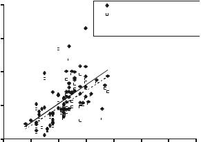
Fig. 10.12 Plot of Cobb-equivalent 1 and Cobb-equivalent 2 angles against clinically measured coronal Cobb angle for each patient in the series. Note that for 10 of the 79 patients, there was only one inflection point on the polynomial curve so Cobb-equivalent1 could not be determined for these ten patients

comparison between the clinically measured (standing) Cobb angle and the Cobbequivalent 1 and Cobb-equivalent 2 metrics derived from the supine CT scans for the patient group.

With respect to Fig. 10.12, the relatively low R2 values of 0.38 and 0.32 (Cobb-equivalent 1 and Cobb-equivalent 2, respectively) show there are substantial variations between individual clinical Cobb measurements from standing radiographs, and the Cobb-equivalent angles derived from continuum representations of spine shape on supine CT scans. The 13.7 and 15.5◦ offsets in the linear regression equations for the two Cobb-equivalent angles are consistent with the magnitude of change in Cobb angle between standing and supine postures of 9◦ and 17◦ reported by Torell et al. [58] and Yazici et al. [59]. The gradients of the regression lines for Cobb-equivalent 1 (1.13) and Cobb-equivalent 2 (1.04) in Fig. 10.13 are close to unity as would be expected, but the slightly greater than unity values suggest that either (1) bigger scoliotic curves are more affected by gravity (i.e. the difference between standing and supine Cobb increases with increasing Cobb angle), or (2) there is greater rotation of the anterior vertebral column (where clinical Cobb angles are measured from endplates) compared to the posterior vertebral canal (where the Cobb-equivalent landmarks are measured) in patients with larger deformities. Note that although not shown in Fig. 10.12, Cobb-equivalent 1 and Cobb-equivalent 2 are highly correlated with each other (R2 = 0.96).

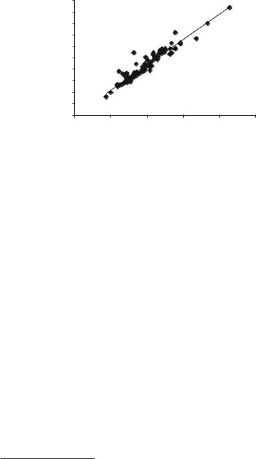
Figure 10.13 shows the close correlation between two of the new metrics, the coronal tortuosity (segmental Ferguson angle) of the major curve and the Cobb-equivalent 2. The coronal tortuosity, M (or segmental Ferguson angle), is strongly correlated (R2 = 0.906, p < 0.0000001) with the Cobb-equivalent 2 angle.

242

Major Coronal Tortuosity (°)

C. Adam and G. Dougherty

100.0
90.0
80.0
70.0				y = 1.0985x
60.0
				R² = 0.9057
50.0
40.0
30.0
20.0
10.0
0.0
0.0	20.0	40.0	60.0	80.0	100.0

Cobb-Equivalent 2 (°)

Fig. 10.13 Major coronal tortuosity (segmental Ferguson angle) vs. Cobb-equivalent 2 for the patient group, showing the close correlation between these two metrics

It is almost 10% larger for all angles, as expected from a metric based on the Ferguson angle, and there is no offset angle. This represents a strong internal consistency for these two semi-automated metrics. M follows the Cobb-equivalent 2 angle in being larger than the measured Cobb angle and having a significant correlation (R2 = 0.30, p < 0.007) to it.

To remove the influence of (1) patient positioning (supine vs. standing) and

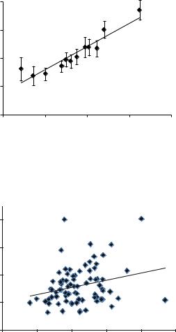
(2) measurement error associated with a single clinical Cobb measurement, we performed a separate sub-study on 12 of the 79 patients in the main patient group.2 For each patient in the sub-study, repeated manual Cobb measurements (six clinicians measured each Cobb angle on three separate occasions at least a week apart) were made using 2D coronal reconstructions from the supine CT scans. This allowed direct comparison of manual and Cobb-equivalent metrics using the same supine CT datasets, and reduced manual measurement variability by using repeated measures by multiple observers. Figure 10.14 shows the result of this comparison.

The R2 value of 0.88 in Fig. 10.14 suggests that when postural differences are accounted for, the Cobb-equivalent metric is strongly correlated to manual Cobb measurements, but has the advantage of not being prone to the substantial manual measurement variability which can occur with a single Cobb measurement by a single observer. Note that the intercept and gradient of the regression equation in Fig. 10.14 suggest that although the metric is strongly correlated with supine manual measures, there is still a difference between the magnitudes of the two Cobb measures, perhaps due to the difference in anatomical location of the landmarks used in each case (manual Cobb uses endplates in the anterior column, whereas

2Note that the measurements described in this sub-study were performed before the main study, so there was no bias in the selection of the 12 patients based on the results from the entire patient group.

10 Applications of Medical Image Processing in the Diagnosis and Treatment...						243
CT	60
supinefromCobbManual reconstructions(°)	50
				y = 0.8192x + 11.37
				R² = 0.8812
	40
	30
	20
	20	30	40	50	60
			Cobb-equivalent 1 (°)

Fig. 10.14 Comparison of manually measured Cobb and Cobb-equivalent 1 for a subgroup of 12 patients, where manual Cobb angles were measured from 2D coronal supine CT reconstructions. Each data point represents the mean of 18 manual measurements (six observers on three occasions each). Error bars are the standard deviation of the manual measurements

tortuosity,	800
rms	600				y = 2.6057x + 208.65
					R² = 0.0642
normalized
	400
	K
Coronal	200
	0
	0.0	20.0	40.0	60.0	80.0	100.0

Coronal tortuosity, M

Fig. 10.15 Plot of normalized root-mean-square tortuosity, K, against tortuosity, M, both measured in the coronal (AP) plane, for each patient in the series

Cobb-equivalent metric uses vertebral canal). Also the number of patients used in this sub-study was relatively small, due to the constraints associated with obtaining multiple repeat Cobb measurements by a group of clinicians.

Figure 10.15 shows the relationship between the two tortuosity-based metrics, K and M (Sect. 10.3.3). Clearly, the correlation is very poor, although both metrics have been shown to correlate well with the ranking of an expert panel when used with retinal vessels [47]. However, in this application, the data is very sparse and there are no ‘data balls’ which can be used to constrain the spline-fitting [45].