10 Applications of Medical Image Processing in the Diagnosis and Treatment...

229

Fig. 10.2 Post-operative X-rays single rod showing anterior (left) and dual rod posterior (right) implants for scoliosis correction

conservative treatment in which the patient is asked to wear an orthotic brace which attempts to exert corrective forces on the deformed spine. Surgical approaches to scoliosis correction (Fig. 10.2) involve attachment of implants to the spine to restore a more normal curvature. Successful surgical approaches typically achieve a 60% reduction of the deformity and prevent further progression; however, there are risks of complication and further deformity progression after surgery which mandate ongoing imaging to monitor the corrected spine.

10.2 Imaging Modalities Used for Spinal Deformity Assessment

Many spinal deformities are visible just by looking at a patient. However, due to differences in body fat levels and bone structure between patients, they cannot be accurately assessed by visual examination of the patient’s appearance. Medical imaging, therefore, plays a key role both in the monitoring of spinal deformity progression before treatment, and in assessing treatment outcomes. There are four medical imaging modalities relevant to the assessment of spinal deformities.

230	C. Adam and G. Dougherty

Planar and biplanar radiography Plane radiographs (X-rays) are the gold standard for imaging spinal deformities, and are used in spine clinics worldwide. A relatively new technology developed in France, the EOS system (EOS imaging, Paris, France), uses bi-planar radiography to simultaneously obtain coronal and sagittal radiographs of standing scoliosis patients with low radiation dose.

Computed Tomography (CT) CT is currently not used routinely for clinical assessment of scoliosis due to its greater cost and higher radiation dose than plane X-rays [1, 2]. However, low dose pre-operative CT is clinically indicated in endoscopic or keyhole scoliosis surgery for planning implant placement [3], and advances in scanner technology now allow CT with much lower radiation doses than previously possible [4]. In the research context, a number of groups have used CT to assess spinal deformities (in particular vertebral rotation in the axial plane) due to the 3D information provided [5–10].

Magnetic Resonance (MR) MR imaging is sometimes used clinically to detect soft tissue abnormalities (particularly the presence of syringomyelia in scoliosis patients), but clinical use of MR for spinal deformities is generally limited. Several research studies have used MR to investigate scoliosis [11–15]. MR is a useful research tool because of the absence of ionizing radiation, although the ability of MR to define bony anatomy is limited and thus image processing of MR datasets is often labour-intensive.

Back surface topography Various optical surface topography systems have been used to directly visualise the cosmetic effects of spinal deformity by assessing back shape in 3D [16–24]. Back surface topography does not involve ionising radiation, and so is useful for functional evaluations involving repeated assessments [25]. However, the relationship between spinal deformity and back shape is complicated by factors such as body positioning, trunk rotation, body build and fat folds [26].

10.2.1 Current Clinical Practice: The Cobb Angle

Currently, the accepted measure for clinical assessment of scoliosis is the Cobb angle [27]. The Cobb angle is measured on plane radiographs by drawing a line through the superior endplate of the superior end vertebra of a scoliotic curve, and another line through the inferior endplate of the inferior-most vertebra of the same scoliotic curve, and then measuring the angle between these lines (Fig. 10.3). Clinically, many Cobb measurements are still performed manually using pencil and ruler on hardcopy X-ray films, but PACS systems (viz. computer networks) are increasingly used which allow manual Cobb measurements to be performed digitally by clinicians on the computer screen. As well as being used to assess scoliosis in the coronal plane, the Cobb angle is used on sagittal plane radiographs to assess thoracic kyphosis and lumbar lordosis.

10 Applications of Medical Image Processing in the Diagnosis and Treatment...

231

Fig. 10.3 Schematic view of a scoliotic deformity showing measurement of the Cobb angle

α

Cobb angle

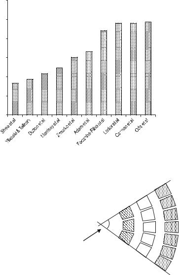
Although widely used for scoliosis assessment for its simplicity, the Cobb angle has several shortcomings. First, numerous studies have shown that the interand intra-observer measurement variabilities associated with the Cobb angle are high. If the vertebral endplates on a plane X-ray appear blurred due to a forward or backward tilt, considerable inter-observer errors can be introduced in the Cobb method as a result of the difficulty in selecting the endplate orientation. Such errors are even more pronounced in the presence of contour changes resulting from osteoporosis [28, 29]. Figure 10.4 shows a summary of Cobb variability studies performed between 1982 and 2005, indicating that the 95% confidence interval for the difference between two measurements by the same observer is around 5–7◦, and for two measurements by different observers is around 6–8◦. These measurement errors are large enough to make the difference between a diagnosis of progression (requiring treatment) or stability, and so introduce uncertainty into the assessment and treatment process.

Second, because of its simplicity, the Cobb angle omits potentially useful information about the shape of a scoliotic spine. Specifically, the Cobb angle cannot differentiate between a large scoliotic curve which may span 8 or 9 vertebral levels, and a small scoliotic curve which may only span 2 or 3 vertebral levels but that has the same endplate angulation due to its severity (Fig. 10.5).

10.2.2 An Alternative: The Ferguson Angle

Prior to the adoption of the Cobb angle as standard practice by the Scoliosis Research Society in 1966, a number of other scoliosis measurement techniques

232

intra-observer variability	(degrees)
95% CI for

C. Adam and G. Dougherty

12

10

8

6

4

2

0

Fig. 10.4 Ninety five percent confidence intervals for intra-observer measurement variability using the Cobb angle from previous studies (figure based on [30])

Fig. 10.5 Simplified representation of three different scoliotic curves with increasing radius and a greater number of vertebral levels in the curve, but the

same Cobb angle	α
	Cobb angle

had been proposed, including the Ferguson angle [31]. The Ferguson angle requires identification of three landmark points, the geometric centres of the upper, apical (i.e. the most laterally deviated) and lower vertebrae in a scoliotic curve (Fig. 10.6). Not only does the Ferguson angle take into account the position of the apical vertebra, which the Cobb angle does not, it is less influenced by changes in the shape of the vertebrae [32].