10	C.L. Luengo Hendriks et al.

If you are a programmer, then such a script is obvious. However, compared to many other languages that require a compilation step, the advantage with MATLAB is that you can select one or a few commands and execute them independently of the rest of the script. You can execute the program line by line, and if the result of one line is not as expected, modify that line and execute it again, without having to run the whole script anew. This leads to huge time savings while developing new algorithms, especially if the input images are large and the analysis takes a lot of time.

2.3 Cervical Cancer and the Pap Smear

Cervical cancer is one of the most common cancers for women, killing about a quarter million women world-wide every year. In the 1940s, Papanicolaou discovered that vaginal smears can be used to detect the disease at an early, curable stage [2]. Such smears have since then commonly been referred to as Pap smears. Screening for cervical cancer has drastically reduced the death rate for this disease in the parts of the world where it has been applied [3]. Mass screens are possible because obtaining the samples is relatively simple and painless, and the equipment needed is inexpensive.

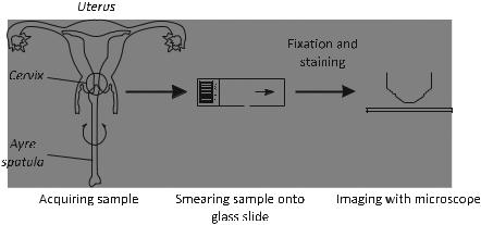
The Pap smear is obtained by collecting cells from the cervix surface (typically using a spatula), and spreading them thinly (by smearing) on a microscope slide (Fig. 2.2). The sample is then stained and analyzed under the microscope by a cytotechnologist. This person needs to scan the whole slide looking for abnormal cells, which is a tedious task because a few thousand microscopic fields of view need to be scrutinized, looking for the potentially few abnormal cells among the

Fig. 2.2 A Pap smear is obtained by thinly smearing collected cells onto a glass microscope slide

2 Rapid Prototyping of Image Analysis Applications

11

several hundred thousand cells that a slide typically contains. This work is made even more difficult due to numerous artifacts: overlapping cells, mucus, blood, etc. The desire to automate the screening has always been great, for all the obvious reasons: trained personnel are expensive, they get tired, their evaluation criteria change over time, etc. The large number of images to analyze for a single slide, together with the artifacts, has made automation a very difficult problem that has occupied numerous image analysis researchers over the decades.

2.4An Interactive, Partial History of Automated Cervical Cytology

This section presents an “interactive history,” meaning that the description of methods is augmented with bits of code that you, the reader, can try out for yourself. This both makes the descriptions easier to follow, and illustrates the use of DIPimage to quickly and easily implement a method from the literature. This section is only a partial history, meaning that we show the highlights but do not attempt to cover everything; we simplify methods to their essence, and focus only on the image analysis techniques, ignoring imaging, classification, etc. For a somewhat more extensive description of the history of this field see for instance the paper by Bengtsson [4].

2.4.1 The 1950s

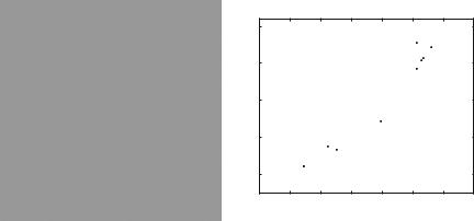
The first attempt at automation of Pap smear assessment was based on the observation that cancer cells are typically bigger, with a greater amount of stained material, than normal cells. Some studies showed that all samples from a patient with cancer had at least some cells with a diameter greater than 12 μm, while no normal cells were that large. And thus a system, the cytoanalyzer, was developed that thresholded the image at a fixed level (Fig. 2.3a), and measured the area (counted the pixels) and the integrated optical density (summed gray values) for each connected component [5]. To replicate this is rather straightforward, and very similar to what we did in Sect. 2.2.3:

a = readim(’papsmear.tif’); b = a<128;

msr = measure(b,a,{’Size’,’Sum’});

As you can see, this only works for very carefully prepared samples. Places where multiple cytoplasms overlap result in improper segmentation, creating false large regions that would be identified as cancerous. Furthermore, the threshold value of 128 that we selected for this image is not necessarily valid for other images. This

12	C.L. Luengo Hendriks et al.

a	b
	integrated optical density (uncalibrated)

x 104

8

7

6

5

4

450 500 550 600 650 700 750 800 area (px2)

Fig. 2.3 (a) Segmented Pap-smear image and (b) plot of measured area vs. integrated optical density

requires strong control over the sample preparation and imaging to make sure the intensities across images are constant.

The pixel size in this machine was about 2 μm, meaning that it looked for segmented regions with a diameter above 6 pixels. For our image this would be about 45 pixels. The resulting data was analyzed as 2D scatter plots and if signals fell in the appropriate region of the plot the specimen was called abnormal (Fig. 2.3b):

figure, plot(msr.size,msr.sum,’.’)

All the processing was done in hardwired, analog, video processing circuits. The machine could have worked if the specimens only contained well-preserved, single, free-lying cells. But the true signal was swamped by false signals from small clumps of cells, blood cells, and other debris [6].

2.4.2 The 1960s

One of the limitations of the cytoanalyzer was the fixed thresholding; it was very sensitive to proper staining and proper system setup. Judith Prewitt (known for her local gradient operator) did careful studies of digitized cell images and came up with the idea of looking at the histogram of the cell image [7]. Although this work was focused on the identification of red blood cells, the method found application in all other kinds of (cell) image analysis, including Pap smear assessment.

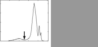
Assuming three regions with different intensity (nucleus, cytoplasm, and background), we would expect three peaks in the histogram (Fig. 2.4a). For simple shapes, we expect fewer pixels on the border between the regions than in the

2 Rapid Prototyping of Image Analysis Applications

13

a							b
of pixels)	2000
	1500
(number	1000
frequency	500
	0	0	50	100	150	200	250
				gray value

Fig. 2.4 (a) Histogram of Pap-smear image, with calculated threshold and (b) segmented image

regions themselves, meaning that there would be two local minima in between these three peaks, corresponding to the gray values of the pixels forming the borders. The two gray values corresponding to these two local minima are therefore good candidates for thresholding the image, thereby classifying each pixel into one of the three classes (Fig. 2.4b). Detecting these two local minima requires simplifying the histogram slightly, for example by a low-pass filter, to remove all the local minima caused by noise:

a = readim(’papsmear.tif’);

h = diphist(a);	% obtain a histogram
h = gaussf(h,3);	% smooth the histogram
t = minima(h);	% detect the local minima
t(h==0) = 0;	% mask out the minima at the tails
t = find(t)	% get coordinates of minima
a < t(1)	% threshold the image at the first
	local minimum

Basically, this method substitutes the fixed threshold of the cytoanalyzer with a smoothing parameter for the histogram. If this smoothing value is taken too small, we find many more than two local minima; if it is too large, we do not find any minima. However, the results are less sensitive to the exact value of this parameter, because a whole range of smoothing values allows the detection of the two minima, and the resulting threshold levels are not affected too much by the smoothing. And, of course, it is possible to write a simple algorithm that finds a smoothing value such that there are exactly two local minima:

h = diphist(a);

% obtain a histogram

t = [0,0,0]; % initialize threshold array while length(t)>2 % repeat until we have 2 local

minima

14	C.L. Luengo Hendriks et al.

a	b	18
		16
	frequency	14
		12
	weighted	10
		8
		6
		4
		2
		0	50	100	150	200	250
		0
				gray value

Fig. 2.5 (a) Gradient magnitude of Pap-smear image and (b) differential histogram computed from the Pap-smear image and its gradient magnitude

h = gaussf(h,1); % (the code inside the loop is identical to that used above)

t = minima(h); t(h==0)=0;

t = find(t);

end

The loop then repeats the original code, smoothing the histogram more and more, until at most two local minima are found.

2.4.3 The 1970s

In the late 1960s, a group at Toshiba, in Japan, started working on developing a Pap smear screening machine they called CYBEST. They used a differential histogram approach for the automated thresholding [8, 9]. That is, they computed a histogram weighted by a measure of edge strength; pixels on edges contribute more strongly to this histogram than pixels in flat areas. Peaks in this histogram indicate gray values that occur often on edges (Fig. 2.5). Though CYBEST used a different scheme to compute edge strength, we will simply use the Gaussian gradient magnitude

(gradmag).

a =	readim(’papsmear.tif’);
b =	gradmag(a);
h =	zeros(255,1);		% initialize array
for	i = 1:255
	t = a==i;	% t is a binary mask
	n = sum(t);	% n counts number of pixels with value i

2 Rapid Prototyping of Image Analysis Applications				15
if n>0
h(i) = sum(b(t))/n;			% average gradient at pixels
			with value i
end
end
h = gaussf(h,2);		% smooth differential histogram
[ ,t] = max(h);		% find location of maximum
a < t	% threshold

A second peak in this histogram gives a threshold to distinguish cytoplasm from background, much like in Prewitt’s method.

This group studied which features were useful for analyzing the slides and ended up using four features [10]: nuclear area, nuclear density, cytoplasmic area, and nuclear/cytoplasmic ratio. These measures can be easily obtained with the measure function as shown before. They also realized that nuclear shape and chromatin pattern were useful parameters but were not able to reliably measure these features automatically, mainly because the automatic focusing was unable to consistently produce images with all the cell nuclei in perfect focus. Nuclear shape was determined as the square of the boundary length divided by the surface area. Determining the boundary length is even more sensitive to a correct segmentation than surface area. The measure function can measure the boundary length (’perimeter’), as well as the shape factor (’p2a’). The shape factor, computed by perimeter2/(4π area), is identical to CYBEST’s nuclear shape measure, except it is normalized to be 1 for a perfect circle. The chromatin pattern measure that was proposed by this group and implemented in CYBEST Model 4 is simply the number of blobs within the nuclear region [11]. For example (using the a and t from above):

m = gaussf(a) < t;				% detect nuclei
m	=	label(m)==3;		% pick one nucleus
m	=	(a < mean(a(m))) & m; % detect regions within
				nucleus
max(label(m))			% count number of regions

Here, we just used the average gray value within the nucleus as the threshold, and counted the connected components (Fig. 2.6). The procedure used in CYBEST was more complex, but not well described in the literature.

The CYBEST system was developed in four generations over two decades, and tested extensively, even in full scale clinical trials, but was not commercially successful.

2.4.4 The 1980s

In the late 1970s and 1980s, several groups in Europe were working on developing systems similar to CYBEST, all based on the so-called “rare event model,” that is,

16	C.L. Luengo Hendriks et al.

Fig. 2.6 A simple chromatin pattern measure: (a) the nucleus, (b) the nucleus mask, and (c) the high-chromatin region mask within that nucleus

looking for the few large, dark, diagnostic cells among the few hundred thousand normal cells. And these systems had to do this sufficiently fast, while avoiding being swamped by false alarms due to misclassifications of overlapping cells and small clumps of various kinds.

As a side effect of the experimentation on feature extraction and classification, carried out as part of this research effort, a new concept emerged. Several groups working in the field observed that even “normal” cells on smears from patients with cancer had statistically significant shifts in their features towards the abnormal cells. Even though these shifts were not strong enough to be useful on the individual cell level, it made it possible to detect abnormal specimens through a statistical analysis of the feature distributions of a small population, a few hundred cells, provided these features were extracted very accurately. This phenomenon came to be known as MAC, malignancy associated changes [12]. The effect was clearly most prominent in the chromatin pattern in the cell nuclei. The CYBEST group had earlier noted that it was very difficult to extract features describing the chromatin pattern reliably in an automated system. A group at the British Colombia Cancer Research Centre in Vancouver took up this idea and developed some very careful cell segmentation and chromatin feature extraction algorithms.

To accurately measure the chromatin pattern, one first needs an accurate delineation of the nucleus. Instead of using a single, global threshold to determine the nuclear boundary, a group in British Colombia used the gradient magnitude to accurately place the object boundary [13]. They start with a rough segmentation, and selected a band around the boundary of the object in which the real boundary must be (Fig. 2.7a):

a = readim(’papsmear.tif’);

b = gaussf(a,2)<128;		% quick-and-dirty threshold
c	= b-berosion(b,1);	% border pixels
c	= bdilation(c,3);	% broader region around border

2 Rapid Prototyping of Image Analysis Applications

17

Fig. 2.7 Accurate delineation of the nucleus: (a) boundary regions, (b) gradient magnitude, (c) upper skeleton, and (d) accurate boundaries

Now comes the interesting part: a conditional erosion that is topology preserving (like the binary skeleton), but processes pixels in order of the gray value of the gradient magnitude (Fig. 2.7b), low gray values first. This implies that the skeleton will lie on the ridges of the gradient magnitude image, rather than on the medial axis of the binary shape. This operation is identical to the upper skeleton or upper thinning, the gray-value equivalent of the skeleton operation [14], except that the latter does not prune terminal branches nor isolated pixels (Fig. 2.7c). We can prune these elements with two additional commands (Fig. 2.7d):

g = gradmag(a);

g = closing(g,5); % reducing number of local minima in g

d= dip upperskeleton2d(g*c);

%compute upper skeleton in border region only

18 C.L. Luengo Hendriks et al.

d	=	bskeleton(d,0,’looseendsaway’);
		% prune terminal branches
d	=	d -getsinglepixel(d);	% prune isolated pixels

It is interesting to note, the upper skeleton is related to the watershed in that both find the ridges of the gray value image. We could have used the function watershed to obtain the exact same result.

We now have an accurate delineation of the contour. The following commands create seeds from the initial segmentation, and grow them to fill the detected contours:

e = b & c;

e = bpropagation(e, d,0,1,0);

Because the pixels comprising the contours are exactly on the object edge, we need an additional step to assign each of these pixels to either the background or the foreground. In the paper, the authors suggest two methods based on the gray value of the pixel, but do not say which one is better. We will use option 1: compare the border pixel’s value to the average for all the nuclei and the average for all the background, and assign it to whichever class it is closest:

gv		nuc = mean(a(e));				% average nuclear gray value
gv		bgr = mean(a( (d|e)));					% average background gray
							value
t = a < (gv nuc+gv					bgr)/2;		% threshold halfway between
							the two averages
e(d) = t(d);			% reassign border pixels only

The other option is to compare each border pixel with background and foreground pixels in the neighborhood, and will likely yield a slightly better result for most cells.

A very large group of features were proposed to describe each nucleus. Based on the outline alone, one can use the mean and maximum radius, sphericity, eccentricity, compactness, elongation, etc., as well as Fourier descriptors [15]. Simple statistics of gray values within one nucleus are maximum, minimum, mean, variance, skewness, and kurtosis. Texture features included contour analysis and region count after thresholding the nucleus into areas of high, medium and low chromatin content; statistics on the co-occurrence matrix [16] and run lengths [17]; and the fractal dimension[18]. The fractal dimension is computed from the fractal area measured at different resolutions, and gives an indication of how the image behavior changes with scale. The fractal area is calculated with:

fs = 1 + abs(dip finitedifference(a,0,’m110’)) + ...

abs(dip finitedifference(a,1,’m110’));

m = label(e)==4;		% pick	one nucleus
sum(fs(m))	% sum values		of fs within nucleus

2 Rapid Prototyping of Image Analysis Applications

19

The function dip finitedifference calculates the difference between neighboring pixels, and is equivalent to MATLAB’s function diff, except it returns an image of the same size as the input.

Multivariate statistical methods were finally used to select the best combination of features to determine whether the cell population was normal or from a slide influenced by cancer.

2.4.5 The 1990s

In the 1990s, research finally lead to successful commercial systems being introduced: AutoPap [19] and PAPNET [20]. They built on much of the earlier research, but two concepts were extensively used in both of these commercial systems: mathematical morphology and neural networks. In short, what the PAPNET systems did was detect the location of nuclei of interest, extract a square region of fixed size around this object, and use that as input to a neural network that classified the object as debris/benign/malignant [21]. Using such a system, these machines avoided the issues of difficulty in segmentation, careful delineation, and accurate measurement. Instead, the neural network does all the work. It is trained with a large collection of nuclei that are manually classified, and is then able to assign new nuclei to one of the classes it was trained for. However, the neural network is a “black box” of sorts, in that it is not possible to know what features of the nucleus it is looking at to make the decision [22]. Slightly simplified, the method to extract fixed-sized image regions containing a nucleus is as follows:

a = readim(’papsmear.tif’);

b = gaussf(a); % slight smoothing of the image

b	=	closing(b,50)-b;	% top-hat, max. diameter is 50
			pixels
c	=	threshold(b);

The closing minus the input image is a top-hat, a morphological operation that eliminates large dark regions. The result, c, is a mask where all the large objects (nuclei clusters, for example) have been removed. But we also want to make sure we only look at objects that are dark in the original image:

c = c & threshold(a);

c now contains only objects that are dark and small (Fig. 2.8a). The next step is to remove the smallest objects and any object without a well-defined edge:

d = gradmag(a,3);
d	= threshold(d);	% detect strong edges
d	= brmedgeobjs( d);	% find inner regions

The first step finds regions of large gradient magnitude. In the second step we invert that mask and remove the part that is connected to the image border.

20	C.L. Luengo Hendriks et al.

Fig. 2.8 Detecting the location of possible nuclei: (a) all dark, small regions, (b) all regions surrounded by strong edges, and (c) the combination of the two

Fig. 2.9 Extracted regions around potential nuclei. These subimages are the input to a neural network

The regions that remain are all surrounded by strong edges (Fig. 2.8b). The combination of the two partial results,

e = c & d;

contains markers for all the medium-sized objects with a strong edge (Fig. 2.8c). These are the objects we want to pass on to the neural network for classification. We shrink these markers to single-pixel dots and extract an area around each dot (Fig. 2.9):

e = bskeleton(e,0,’looseendsaway’);

% reduce each region to a single dot

coords = findcoord(e);	%get the coordinates for each
	dot

N = size(coords,1); % number of dots

reg = cell(N); % we’ll store the little regions in here for ii=1:N

x = coords(ii,1); y = coords(ii,2);

reg{ii} = a(x-20:x+20,y-20:y+20);

% the indexing cuts a region from the image

end

reg = cat(1,reg{:}) % glue regions together for display

2 Rapid Prototyping of Image Analysis Applications

21

That last command just glues all the small regions together for display. Note that, for simplicity, we did not check the coords array to avoid out-of-bounds indexing when extracting the regions. One would probably want to exclude regions that fall partially outside the image.

The PAPNET system recorded the 64 most “malignant looking” regions of the slide for human inspection and verification, in a similar way to what we did just for our single image field.

2.4.6 The 2000s

There was a reduced academic research activity in the field after the commercial developments took over in the 1990s. But there was clearly room for improvements, so some groups continued basic research. This period is marked by the departure from the “black box” solutions, and a return to accurate measurements of specific cellular and nuclear features. One particularly active group was located in Brisbane, Australia [23]. They applied several more modern concepts to the Pap smears and demonstrated that improved results could be achieved. For instance, they took the dynamic contour concept (better known as the “snake,” see Chapter 4) and applied it to cell segmentation [24]. Their snake algorithm is rather complex, since they used a method to find the optimal solution to the equation, rather than the iterative approach usually associated with snakes, which can get stuck in local minima. Using “normal” snakes, one can refine nuclear boundary thus:

a = readim(’papsmear.tif’)

b = bopening(threshold(-a),5); % quick-and-dirty

%segmentation
c = label(b);	% label the nuclei
N = max(c);	% number of nuclei
s = cell(N,1);	% this will hold all snakes
vf = vfc(gradmag(a));		% this is the snake’s ‘‘external
			force’’
for ii = 1:N	% we compute the snake for each nucleus
	separately
ini = im2snake(c==ii);			% initial snake given by
			segmentation

s{ii} = snakeminimize(ini,vf,0.1,2,1,0,10); % move snake so its energy is minimized

snakedraw(s{ii}) % overlays the snake on the image

end

The snake is initialized by a rough segmentation of the nuclei (Fig. 2.10a), then refined by an iterative energy minimization procedure (snakeminimize, Fig. 2.10b). Note that we used the function vfc to compute the external force, the image that drives the snake towards the edges of the objects. This VFC (vector field