198	M.A. Haidekker and G. Dougherty

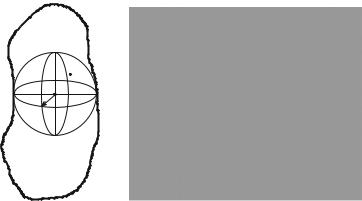
Fig. 9.2 Cross-sectional magnetic resonance image of a human forearm. Similar to Fig. 9.1, radius and ulna can easily be recognized. In contrast to the CT image, however, compact bone appears dark, and the MR image clearly reveals soft tissue features, such as muscle, tendons, and blood vessels. Spongy bone appears particularly bright because of the long relaxation times of bone marrow. The inset shows the section inside the white rectangle magnified and inverted to match the higher image values for bone in CT images. In the spongy area, texture that is related to trabecular structure is discernible, although it appears more blurred than in the corresponding CT image. Image courtesy of Dr. Kai Haidekker

the ratio of the transmitted spectra with and without the sample. A single value, often referred to as BUA (the broadband ultrasound attenuation value), is obtained from the slope of the attenuation over the frequency. No theoretical relationship between ultrasound attenuation and the mechanical properties of cancellous bone has been established [24], but both the speed of sound and the BUA value are higher in healthy bone than in osteoporotic bone.

9.3 Quantifying the Microarchitecture of Trabecular Bone

In Sect. 9.1, we discussed the need to estimate the individual fracture risk and the role that bone microstructure plays in that estimation. A very rigorous approach is computerized modeling of the biomechanical behavior of bone under a defined load. For this purpose, the exact three-dimensional microscopic geometry of the trabeculae and their interface with cortical bone need to be available. It is feasible to extract the geometry with sufficient precision by micro-CT or microscopy or

9 Medical Imaging in the Diagnosis of Osteoporosis...

199

histology in a slice-by-slice manner [25], yet these methods are normally restricted to ex vivo samples. Other three-dimensional imaging methods with high resolution, for example, micro-MRI, change the apparent geometry due to the system’s pointspread function. At lower resolution, individual trabeculae cannot be imaged accurately. In such cases, the image shows a distinct texture that is more or less related to trabecular microarchitecture. Even two-dimensional cross-sectional slices and projection images can provide such texture information, but other influences (noise, reconstruction artifacts, pseudo-texture) become more dominant as the resolution becomes lower. Below a certain resolution, artifacts dominate, and any texture in the image is unrelated to trabecular microarchitecture, at which the image can only be used to measure average bone density. The most important methods to quantify image texture and relate it to trabecular microarchitecture are discussed in this section.

9.3.1 Bone Morphometric Quantities

Morphometric quantities are directly related to the microstructure of the trabecular network. From the segmented three-dimensional bone image, total volume and bone surface area can be obtained immediately. In the literature [26], these are abbreviated TV and BS, respectively. Bone volume (BV) is the space occupied by actual bone mineral. BV can be determined by measuring the total volume of the trabeculae after segmentation of those voxels that lie above a certain density. These primary indices can be used in normalized form, that is, relative bone volume BV/TV, relative bone surface BS/TV, and bone surface–volume-ratio BS/BV, to allow comparison between individuals.

Microstructural analysis of the trabeculae leads to the derived indices of trabecular thickness (Tb.Th) and trabecular spacing (Tb.Sp). In a simplified model, trabeculae can be interpreted as thin plates of constant thickness and width. In this case, the following relationships can be found [27]:

T b.T h = 2BV /BS
T b.Sp = 2(BV − TV )/BS
T b.N = BS/2BV	(9.3)

Tb.N is the number of trabecular plates. Bone mineral content (BMC) was found to directly correlate with the normalized bone volume [28],

	BMC =	BV	ρBα	(9.4)
		TV

where ρB is the specific weight of bone mineral and α is the ash fraction. Values for α range from α = 0 for osteoid to α = 0.7 for fully mineralized bone [28].

200	M.A. Haidekker and G. Dougherty
a	b

P

r

Ω

Fig. 9.3 Analysis of the trabecular microstructure. (a): Structures can be quantitatively analyzed by fitting a maximum-radius sphere into the structure Ω so that a point P Ω is an element of the maximum-radius sphere (adapted from [29]). (b): Scan-line method to quantify the microstructure. Parfitt [26] suggested counting the intersections of the bone structure with a rectangular grid of lines to obtain Tb.N. The method can be extended to obtain the distribution of runs along bone (light gray) and runs along marrow spaces (black)

These values correspond to a dry tissue density of 1.41 g/cm3 and 2.31 g/cm3, respectively. Furthermore, an experimental relationship of these values to elasticity E and ultimate stress σult was found (9.5) with the constants a, b, c, and d determined by nonlinear regression as a = 2.58 ± 0.02, b = 2.74 ± 0.13, c = 1.92 ± 0.02, and d = 2.79 ± 0.09 [28].

E (BV /TV )aα b;

σult (BV /TV )cα d

(9.5)

The assumption of homogeneous plates is a very rough approximation, and actual measurements from images provide more accurate estimations. Hilebrand and R¨uegsegger proposed an image analysis method where a maximum-size sphere is fitted into the space between the segmented trabeculae [29]. By examining each point P inside the structure (Fig. 9.3a), statistical analysis of the void spaces can be performed. For each structure, the mean thickness (the arithmetic mean value of the local thicknesses taken over all points in the structure), the maximum thickness, average volume, and similar metrics can be found and examined over the entire bone segment, which can then be characterized by statistical methods. This method is capable of analyzing 3D volumetric data, but by using a circle rather than a sphere, it can be adapted to 2D slices.

An alternative method, known as the run-length method, can produce similar quantitative parameters with relatively low computational effort. Originally, Parfitt [26] suggested to use a rectangular grid of scanlines and count the intersections with trabecular bone in microscopic images to determine Tb.N. This idea can be extended to the run-length method (Fig. 9.3b): In an image that contains the segmented bone,

9 Medical Imaging in the Diagnosis of Osteoporosis...

201

linear runs of bone and marrow are measured. The average length of the marrow runs is related to Tb.Sp, and the average length of the bone runs is related to Tb.Th. The number of bone runs relative to the total number of runs provides Tb.N. With progressing bone deterioration, where trabeculae become thinner and disconnected, we can expect fewer and longer marrow runs, and shorter bone runs. Typically, runs are calculated at 0◦, 45◦, 90◦, and 135◦, and the resulting run lengths are averaged to obtain a measurement that is widely orientation-independent. Alternatively, runs in different directions can be used to determine orientational preferences. The run length method is a 2D method.

Two representative examples for the application of the run-length method for the quantification of trabecular microstructure on CT images [30, 31] demonstrate that this technique does not require an accurate microscopic representation of trabecular bone. A relationship between morphometric quantities and bone strength has been established [32]. On the other hand, noise and partial-volume effects have a strong influence on which voxels are classified as bone. Furthermore, image degradation by the point-spread function of the device makes the selection of a suitable threshold for the separation of bone and soft tissue difficult. Even with micro-CT and micro-MRI techniques, the thickness of individual trabeculae is on the order of a single voxel.

Topological quantities, such as the number of struts or the number of holes, are popular in the analysis of the trabecular network. The interconnected trabeculae can be represented as a graph, and the number of links (i.e., trabecular struts), the number of nodes, the number of holes (i.e., the marrow spaces), and related metrics, such as the Euler characteristic can be determined. The Euler characteristic can be seen as the number of marrow cavities completely surrounded by bone. To obtain the topological quantities, the image needs to be segmented into bone and non-bone areas followed by thinning of the structures (skeletonization, Fig. 9.4). One of the most interesting features of the topological quantities is the invariance under affine transformations. Therefore, these quantities should be robust – within limitations of the pixel discretization – against changes in scale, rotations, and even shear and perspective distortions.

Analysis of the skeleton is traditionally a 2D method, but extensions to 3D have been reported [33]. In two and three dimensions additional parameters have been defined. These include the connectivity index by Le et al. [34]; the marrow star volume by Vesterby et al. [35], which also reflects connectivity; the trabecular bone pattern factor (often abbreviated TBPf ) by Hahn et al. [36], which decreases with bone deterioration; the ridge number density by Laib et al. [37]; and the structure model index (SMI) by Hildebrand and R¨uegsegger [38], which is designed to characterize a 3D shape as being plate-like or rod-like and requires a 3D image of microscopic resolution.

9.3.2 Texture Analysis

Whereas morphometric analysis is based on the assumption that individual trabeculae are resolved in the image (thus, requiring high-resolution images with voxel

202	M.A. Haidekker and G. Dougherty

Fig. 9.4 X-ray image of an excised section of trabecular bone with its skeleton superimposed. Skeletonization is a popular method to quantify the connectivity. Microstructural deterioration of bone increases the number of branches (links that are connected to the network on only one end), and decreases the number of loops

sizes generally smaller than trabecular width), such an assumption is not needed for the analysis of the texture in image regions representing trabecular bone. Texture can be defined as a systematic local variation of the image values [39]. This definition normally implies the existence of multiple image values (gray values) as opposed to the purely binary values used in the morphometric analysis. Moreover, an assumption must be made that the image texture is related to the microstructure of trabecular bone. This is a reasonable assumption, as can be demonstrated in a simple experiment (Fig. 9.5). Let us consider an imaging device with a non-ideal point-spread function, for example, X-ray projection imaging where the size of the focal spot of the X-ray tube and the bone–film distance introduce blur. This process can be simulated by additive superposition of blurred images of some defined binary structure. A structure that somewhat resembles the distribution of trabecular bone is shown in Fig. 9.5a. The purely binary image represents trabecular bone (white) and marrow space (black). This image has been generated by a suitable random generator. Six such images, blurred with a second-order Butterworth filter adjusted to a random cutoff frequency of 10 ± 3 pixel−1 were created and added on a pixel- by-pixel basis (Fig. 9.5b). The similarity of the resulting texture to an actual CT image (Fig. 9.5c) is striking.

9 Medical Imaging in the Diagnosis of Osteoporosis...

203

Fig. 9.5 Demonstration of the relationship between microarchitecture and texture in an imaging system with non-ideal point-spread function. (a): A synthetically generated pattern that somewhat resembles segmented and binarized trabeculae in a microscopic image. (b): Six patterns similar to the one shown in (a), blurred and superimposed. (c): Magnified computed tomography slice of the trabecular area in a lumbar vertebra. The trabecular area has been slightly contrast-enhanced, leading to saturation of the image values that correspond to cortical bone

Texture can be analyzed in two or three dimensions. Because most imaging modalities have anisotropic voxel sizes with much lower resolution in the axial direction than in-plane, texture analysis normally takes place as a two-dimensional operation. In 3D imaging modalities (CT and MRI), texture analysis can take place slice-by-slice. When an analysis method is extended into three dimensions, a possible voxel anisotropy needs to be taken into account.

The simplest method for texture analysis is the computation of the statistical moments of the histogram inside a region of interest. Most notably, the standard deviation and its normalized equivalent, the coefficient of variation, contain information about the irregularity of the structure. Healthy bone can be expected to have a more irregular structure with a higher coefficient of variation than osteoporotic bone with larger and more homogeneous marrow spaces. Both variance and coefficient of variation can be computed locally inside a sliding window. A compact metric is the average local variance (ALV), which shows a similar trend as the global variance, i.e., declines with the lower roughness of the texture of osteoporotic bone. Basic statistical moments can also be computed on gradient images [40], and the first moment is sometimes referred to as edgeness. The use of edge enhancement to emphasize the roughness was applied by Caldwell et al. [41], who processed digitized radiographies of thoracic vertebrae with the Sobel operator and a thresholding algorithm to remove small gradients that are likely caused by noise. A histogram of the gradient values showed two maxima that were related to a preferredly horizontal and vertical orientation of the trabeculae, respectively. The two maxima, relative to the mean gradient, related to the fracture load.

The run length method, introduced in the previous section, can be adapted to analyze texture in a straightforward manner. The grayscale image (such as Fig. 9.5c can be binarized with the application of a threshold. Clearly, the application of a

204	M.A. Haidekker and G. Dougherty

threshold leads to a loss of information, and the original microstructure cannot be restored. The binary run length method can be extended by allowing more than two gray level bins. In this case, a two-dimensional histogram N(g, l) of the number of runs N as a function of the gray value g and the run length l is obtained. The runlength histogram is still relatively complex, and statistical quantities can be extracted that characterize the histogram. Examples are the shortand long-run emphasis (SRE and LRE), low and high gray value emphasis (LGRE and HGRE), combined metrics, such as the long-run low gray-value emphasis (LRLGE), and uniformity metrics, such as the gray-level and run-length nonuniformities (GNLU and RLNU). Three of these quantitative descriptors are listed in (9.6) as examples, and a complete list can be found in [39].

SRE

LGRE

GLNU

G−1 L	P(g, l)
= ∑ ∑
	l2
g=0 l=1
G−1 L	P(g, l)
= ∑ ∑
	(g + 1)2
g=0 l=1
L G−1			2
= ∑ ∑ P(g, l)			(9.6)

l=1 g=0

Here, L is the longest run, G is the number of gray bins, and P(g, l) is the run probability where P(g, l) = N(g, l)/n with n being the total number of runs. It can be expected that trabecular rarefaction due to osteoporosis would increase LRE and LRLGE because of the longer intratrabecular runs, and would decrease GLNU as an indicator of the loss of complexity. In fact, Chappard et al. found that X-ray based SRE and GLN showed a high negative correlation with 2D histomorphometric methods ex vivo. Lespessailles et al. found significant differences in the SRE value between patients with and without osteoporosis-related fractures in a multicenter study [42]. In radiography images, Ito et al. [31] reported a significant increase of a parameter termed I-texture with age and with the presence of fractures. The I-texture is the average length of dark runs in a binary run-length histogram and corresponds to intratrabecular spaces. Conversely, the T-texture, the white runs that correspond to the trabecular area, did not change significantly. This observation can be interpreted as the increase of marrow spaces with otherwise unchanged trabecular width.

Selection of the threshold, or placement of the gray-level bins, have a strong influence on the quantitative texture descriptors. Neither projection images nor CT images allow the application of a defined threshold to separate bone from soft tissue and marrow. Depending on the threshold, the runs can be almost arbitrarily shifted from black to white runs. Bin selection is less critical when a gray-level run-length histogram is computed. However, a large number of gray levels leads to predominantly short runs, whereas a small number of gray levels allows longer runs, but introduces a sensitivity against shifts in image value. Frequently, the bin size b is determined from the maximum and minimum image intensity as

9 Medical Imaging in the Diagnosis of Osteoporosis...

205

b = (Imax − Imin)/G. A few outlier pixels can strongly influence bin placement. In the example of Fig. 9.5b, clamping the brightest 0.1% of the pixels reduces SRE by 15%, LGRE by 25%, GLNU by 28%, SRLGE by 27%, and LRLGE by 16%. All other descriptors are also affected, albeit to a lesser degree. A more robust method to select a threshold or to place bins would be based on the gray-value histogram [43]. Histogram-based threshold and bin selection also ensures that the quantitative descriptors are independent of the image intensity. Bone deterioration leads to lower image values in X-ray and CT images. A change in exposure or a different CT calibration may have a similar effect, although the microstructure has not been altered. The quantitative descriptors directly reflect the image intensity rather than the microarchitecture. This potential fallacy applies to most other texture analysis methods as well. Any method can be subjected to a simple test. If all image values are linearly transformed such that I (x, y) = a · I(x, y) + b, where a > 0 and b are scalars, any algorithm that produces different descriptors for I when a and b are modified does not reflect pure texture.

Other artifacts that may influence texture descriptors are image noise and pseudotexture, introduced in the image formation process. Noise can be seen as an artifactual texture on the pixel level. By using a low number of gray-value bins and by discarding the shortest runs, the run-length method can be made more robust against noise. Pseudo-texture (see, for example, Fig. 9.1) cannot be fully eliminated. In special cases, suitable filters can suppress the pseudo-texture to some extent. The presence of this artifact makes it difficult to compare quantitative parameters obtained with different instruments or reconstruction settings. Lastly, the application of a highpass filter is advisable before texture parameters are determined. A highpass filter removes broad trends in the image values, for example, inhomogeneous X-ray illumination or MR bias field artifacts.

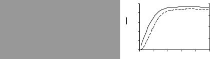
Two other texture analysis methods, based on the co-occurrence matrix [44] and on Law’s texture energy metrics [45], have been successfully applied in texture analysis of trabecular bone. The co-occurrence matrix is the histogram of probabilities that an image value i is accompanied by the image value j at the distance r. To create the co-occurrence matrix, a copy of the image is shifted by −r = ( x, y), and the two-dimensional joint histogram is computed. Analogous to the two-dimensional run-length histogram, single-value quantitative descriptors can be extracted. The most widely used set of quantitative descriptors are known as Haralick’s texture classification metrics [44]. Haralick proposes 14 different classification metrics, such as the energy, entropy, contrast, and correlation. Each of these metrics can be determined for different r. Texture analysis is often driven by a high-dimensional feature vector that is used as the input of some artificialintelligence decision mechanism. In the analysis of bone, however, single values are normally used. The choice of r is critical. Since the texture features of interest are normally larger than a single pixel, single-pixel offsets reflect predominantly noise. A thorough analysis of the relevant size of the features is necessary to obtain meaningful values from the co-occurrence matrix. The influence of the offset r is shown in Fig. 9.6, where the co-occurrence matrices for x = 1 and x = 15

206	M.A. Haidekker and G. Dougherty

a	b	c
		2500					40
		2000					10	)Contrast(----
		Inertia()
							30
		1500					20
		1000
		500
		0					0
		0	10	20	30	40	50
				x (pixels)

Fig. 9.6 Examples of the gray-level co-occurrence matrix of the image in Fig. 9.5b. A singlepixel offset (a) shows highly correlated pixel values with high-probability co-occurrences arranged along the diagonal i = j. With a larger offset ( x = 15 pixels), a broader distribution of the cooccurrence matrix is seen (b). Analysis of the influence of the offset ((c), inertia and contrast shown as representative metrics) reveals that the values strongly depend on the choice of x until x 20

are juxtaposed, and two representative metrics, inertia and contrast, are shown for different x. Neighboring pixels are highly correlated for small r (the diagonal i = j dominates the histogram). The metrics become robust against changes of x for x 20, which indicates that the features of interest coincide with this size. In fact, Euclidean distances between local maxima of the image fluctuate between 15 and 35. One example study be Lee et al. [46] examines the inverse difference moment

IDM (9.7) of the co-occurrence matrix,

	IDM(θ , d) = ∑	Pθ ,d (a, b)	(9.7)
		|a − b|2
	a,b,a =b

where θ and d describe the displacement in polar coordinates, and a and b are the indices of the co-occurrence matrix. Lee et al. found a negative correlation of IDM in digitized radiographies of the femoral neck with bone strength, and found that IDM was significantly correlated with bone density, although highpass filtering and histogram normalization made IDM independent from radiographic density. On the other hand, Lee et al. [46] did not find a statistically significant difference of IDM between cases with and without fractures. One possible reason is the low resolution of approximately 8 pixels/mm, where the displacement d = 7 corresponds to 1 mm and is much larger than the trabecular size. Lespessailles et al. [47] found only a weak and nonsignificant correlation between the energy parameter and bone density. This observation can be interpreted in two ways. First, it should be expected that microarchitectural organization and density are independent quantities, and a high correlation cannot be expected. On the other hand, it is known that microarchitectural deterioration is seen as reduced bone density in large-volume averages, and a moderate correlation between the two quantities should be observed. Since Lespessailles et al. used single-pixel distances for r, the energy metric may have been dominated by pixel noise rather than actual microstructural information.