10 Applications of Medical Image Processing in the Diagnosis and Treatment...

237

metric. Here, we propose that the z-coordinates of the upper and lower end vertebrae of the scoliotic curve as determined clinically are used in this situation. The angle between the normals to the coronal curve at these vertebral levels is again a Cobbequivalent measure, with the disadvantage that a manual selection of levels was required.

The two approaches just presented; (1) Cobb-equivalent angle determined as the angle between inflection points of coronal polynomial, and (2) Cobb-equivalent angle determined as the angle between manually selected vertebral locations of coronal polynomial are denoted as the ‘Cobb-equivalent 1’ and ‘Cobb-equivalent 2’ angles, respectively.

10.3.3 Tortuosity

The concept of tortuosity, the accumulation of curvature along a curve, has been used to characterise blood vessels and their risk of aneurysm formation or rupture [33, 42–47]. A variety of possible metrics for tortuosity have been proposed, such as the distance factor (the relative length increase from a straight line) [48–50] or sinuosity [51], the number of inflection points along the curve [52], the angle change along segments [53,54], and various line integrals of local curvature values [42,44], which can be computed from second differences of the curve [43].

We have developed two tortuosity metrics [45] which are amenable to automation and can be used as putative scoliosis metrics for measuring the severity of the condition. Both are inherently three-dimensional, although they can be applied to two-dimensional projections. (A third possible metric, the integral of the square of the derivative of curvature of a spline-fit smoothest path, was found not to be scaleinvariant, and subsequently abandoned [55]).

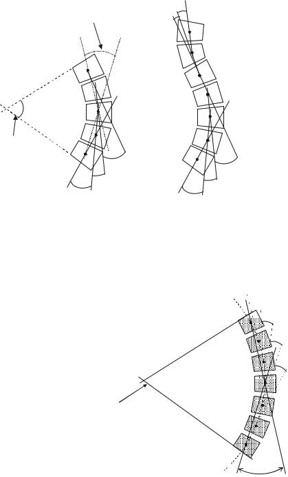
The first metric delivers a scoliotic angle, which can be considered an extension of the Ferguson angle. It is the accumulated angle turned along the length of the section of spine of interest, calculated as the sum of the magnitudes of the angles between straight line segments connecting the consecutive centres of all the vertebrae under consideration (Fig. 10.9). We have previously designated it as M. It can be applied to the whole spine, or a designated curve within it.

Figure 10.9 shows that M can be considered an extension of the Ferguson angle (referred to here as the segmental Ferguson angle). For a given scoliotic curve, the segmental Ferguson angle will be larger than the conventional Ferguson angle and smaller than the Cobb angle, although in the special (theoretical) case of a circular arc comprising many short segments its value approaches that of the Cobb angle. This special case is shown schematically in Fig. 10.10.

The second metric is based on a continuum function for the spinal curve, based on a unit speed parameterization of the vertebral centres. A piece-wise spline is used to produce a continuous function, which is the ‘smoothest path’ connecting the vertebral centres (Fig. 10.11), and it is used to compute a normalized

238		C. Adam and G. Dougherty
Conventional	φ4	φ5
Ferguson angle

Μ=φ1+φ2+φ3

α

Cobb angle

	φ3	φ3
φ2
		φ2
φ1
		φ1
Segmental

Ferguson angles M= |f1|+|f2|+|f3|+|f4|+|f5|

Fig. 10.9 Left: Portion of a scoliotic curve showing conventional Cobb and Ferguson angles as well as the segmental Ferguson angles which are summed to give the coronal tortuosity metric M. Right: Absolute segmental angles are summed in the case of a spinal curve containing both positive and negative angles

Fig. 10.10 For the special case of a circular arc the Cobb angle α is twice the Ferguson angle φ. As the arc is divided into successively more segments, the coronal tortuosity (sum of the

segmental Ferguson angles

M = φ1 + φ2 + φ3 + . . .) approaches the Cobb angle

a = 60°

Cobb angle

f1=f2=f3=f4=f5=8.57° M=f1+f2+f3+f4+f5=42.85°

f5 f4

f3

f2

f1

f =30°

10 Applications of Medical Image Processing in the Diagnosis and Treatment...

239

Fig. 10.11

Anterior–posterior (AP) radiograph, illustrating the measurement of the conventional Cobb and Ferguson angles, and showing the smoothest-path piece-wise spline iteratively fitted to the geometric centres of the vertebrae

root-mean-square (rms) curvature, which we designated K. It is defined in terms of the root-mean-square curvature, J, of the smoothest path by

K =	√	(10.4)
	J.L,

√

where L is the length of the smoothed curve. The ‘normalization’ by L ensures that K is dimensionless (viz. an angle). While M is an accumulated angle using straight line segments between the vertebral centres, K is an accumulated angle using the smoothest path connecting the centres. With K, the accumulation is not democratic; rather contributions of higher curvature are given more weight than contributions of lower curvature. (If the curvature is constant, then K is forced to accumulate democratically and K = M.)

Both metrics have been shown to be scale invariant and additive, and K is essentially insensitive to digitization errors [45] Their usefulness has been demonstrated in discriminating between arteries of different tortuosities in assessing the relative utility of the arteries for endoluminal repair of aneurysms [33].