Multidimensional Chromatography

150	Multidimensional Chromatography

46.S. F. Y. Li, Capillary Electrophoresis. Principles, Practice and Applications, Elsevier, Amsterdam (1992).

47.B. Chankvetadze, Capillary Electrophoresis in Chiral Analysis, John Wiley & Sons, New York (1997).

48.M. G. Cikalo, K. D. Bartle, M. M. Robson, P. Myers and M. R. Euerby, ‘Capillary electrochromatography’, Analyst 123: 87R – 102R (1998).

49.C. Fujimoto, ‘Packing materials and separation efficiencies in capillary electrochromatography’, Trends Anal. Chem. 18: 291 – 301 (1999).

50.K. D. Altria, ‘Overview of capillary electrophoresis and capillary electrochromatography’, J. Chromatogr. 856: 443 – 463 (1999).

51.J. Viudevogel and P. Saundre, ‘Introduction to unicellar electrokinetic chromatography’, Hüthig Verlag GmbH Heidelberg, Germany (1992).

52.S. Terabe, ‘Electrokinetic chromatography: an interface between electrophoresis and chromatography’, Trends Anal. Chem. 8: 129 – 134 (1989).

53.J. P. Landers (Ed.), Handbook of Capillary Electrophoresis, 2nd Edn, CRC Press, Boca Raton, FL (1996).

54.A. J. Tomlinson and S. Naylor, ‘Enhanced performance membrane preconcentration – capillary electrophoresis – mass spectrometry (mPC – CE – MS) in conjunction with transient isotachophoresis for analysis of peptide mixtures, J. High Resolut. Chromatogr. 18: 384 – 386 (1995).

55.A. J. Tomlinson and S. Naylor, ‘Systematic development of on-line membrane preconcentration – capillary electrophoresis – mass spectrometry for analysis of peptide mixtures, J. Capillary Electrophoresis 2: 225 – 233 (1995).

56.N. Guzman, On-line bioaffinity, molecular recognition and preconcentration in CE technology’, LC – GC, 17: 16 (1999).

57.N. M. Djordjevic and K. Ryan, ‘An easy way to enhance absorbance detection on Waters Quanta-4000 capillary electrophoresis system’, J. Liq. Chromatogr. 19: 201 – 206 (1996).

58.F. M. Lanças and M. A. Ruggiero, ‘On-line coupling of supercritical fluid extraction to capillary column electrodriven separation techniques’, J. Microcolumn Sep. 12: 61 – 67 (2000).

59.M. A. Ruggiero and F. M. Lanças, ‘On-line supercritical fluid extraction–capillary electrophoresis (SFE – CE) analysis: development and applications’, in Proceedings of the 20th International Symposium on Capillary Chromatography, Riva del Garda, Italy, May 26 – 29, Sandra P (Ed.), Hüthig, Hedelberg, pp. 22 – 23 (1998).

60.M. A. Ruggiero and F. M. Lanças, ‘Approaching the ideal system for the complete automation in trace analysis by capillary electrophoresis’, in Proceedings of the 3rd Latin American Symposium on Capillary Electrophoresis, Buenos Aires, Argentine, November 30 – December 2. p. 1 (1997).

61.J. C. Giddings, Dynamics of Chromatography. Part I: Principles and Theory, Marcel Dekker, New York (1965).

62.D. Ishii, T. Niwa, K. Ohta and T. Takeuchi, ‘Unified capillary chromatography’, J. High Resolut. Chromatogr. 11: 800 – 801 (1988).

63.K. D. Bartle, I. L. Davies, M. W. Raynor, A. A. Clifford and J. P. Kithinji, ‘Unified multidimensional microcolumn chromatography’, J. Microcolumn Sep. 1: 63 – 70 (1989).

64.D. Tong, K. D. Bartle and A. A. Clifford, ‘Principles and applications of unified chromatography’, J. Chromatogr. 703: 17 – 35 (1995).

65.F. M. Lanças GC SFC LC: Towards unified chromatography’, in Proceedings of the 6th Latin American Congress on Chromatography (COLACRO VI), Caracas, Venezuela Intevep Ed, 25 – P1 (1996).

Multidimensional Chromatography

Edited by Luigi Mondello, Alastair C. Lewis and Keith D. Bartle

Copyright © 2002 John Wiley & Sons Ltd

ISBNs: 0-471-98869-3 (Hardback); 0-470-84577-5 (Electronic)

7Unified Chromatography: Concepts and Considerations for Multidimensional Chromatography

T. L. CHESTER

The Procter & Gamble Company, Cincinnati, OH, USA

7.1INTRODUCTION

Multidimensional chromatography brings together separations often based on different selectivity mechanisms. Although the forms of the mobile phase are not required to be different in the individual steps of a multidimensional separation, we usually strive to achieve orthogonal selectivity of these individual separation steps (1).

This is usually not a problem when bringing together two techniques with very different mobile phases, such as liquid chromatography (LC) and gas chromatography (GC), for example, to carry out a two-dimensional LC–GC separation. In GC, the only significant intermolecular forces are between the solutes and the stationary phase, and there are no attractive forces of any consequence involving the mobile phase. Rather, it is just an inert carrier that transports the gaseous fraction of the solute through the interparticle volume of the column whenever the solute is not associated with the stationary phase. Once a GC column is chosen, control of solute partitioning between the stationary and mobile phases is simply a function of temperature and nothing else.

However, in LC solutes are partitioned according to a more complicated balance among various attractive forces: solutes interact with both mobile-phase molecules and stationary-phase molecules (or stationary-phase pendant groups), the stationaryphase interacts with mobile-phase molecules, parts of the stationary phase may interact with each other, and mobile-phase molecules interact with each other. Cavity formation in the mobile phase, overcoming the attractive forces of the mobile-phase molecules for each other, is an important consideration in LC but not in GC. Therefore, even though LC and GC share a considerable amount of basic theory, the mechanisms are very different on a molecular level. This translates into conditions that are very different on a practical level; so different, in fact, that separate instruments are required in modern practice.

152	Multidimensional Chromatography

Why are these techniques so different, and how did this division of practice arise? Helium and hydrogen are used in GC in preference to other mobile-phase gases because of diffusion. Since there are no interactions involving the mobile phase, gases with the fastest diffusion rates produce analyses in the shortest times. Tswett and the other pioneers of LC chose from among a few convenient liquids to use as mobile phases. These liquids had to have several important features. They could not be so viscous that they would not flow through packed columns by gravity or with the application of modest pressure. They could not be so volatile that they would evaporate before reaching the column outlet. In short, they had to be well-behaved liquids.

This thinking has carried through to the present day and is reflected in our choices of mobile-phase fluids in LC: water, acetonitrile, methanol, tetrahydrofuran, hexane, etc., are still among our popular choices. However, these particular materials are completely dependent on the conditions of column temperature and outlet pressure. Tswett’s original conditions at his column outlet, actually the earth-bound defaults we call ambient temperature and pressure, determined his solvent choices and continue to dominate our thinking today.

If our ambient conditions were different from what they actually are, then we would surely have a much different list of our favorite liquid solvents. Unified chromatography begins with the simple notion of rejecting ambient temperature and outlet pressure as being necessarily correct. Instead, we simply include these parameters with the other chromatographic variables and find the best values of all the parameters, taken together, to accomplish our separation goals. This simple notion leads to a greatly expanded list of possible mobile phases. It also leads to new and different chromatographic performance characteristics that may be of great utility in trying to achieve orthogonality in multidimensional separations.

The history of unified thinking has been driven by a few pioneers. Martire was among the first to address theoretical aspects (2 –7). His unified theory of chromatography spans a variety of mobile-phase conditions from a thermodynamics and statistical mechanics standpoint. Ishii and Takeuchi built instruments that could perform GC, supercritical fluid chromatography (SFC), and LC, usually in discontinuous steps involving a change in mobile phase (8, 9). From this came the concept Ishii called Troika, after the Russian carriage drawn by three horses (GC, SFC, LC). Bartle’s group also contributed developments in instrumentation aimed primarily at performing multiple separation modes sequentially (10 –15). Beginning in the 1960s, Giddings and co-workers did a great deal of work using dense-gas and super- critical-fluid mobile phases. Although Giddings’ research focus turned to field flow fractionation later in his career, his philosophical influence toward thinking about the common or unified traits of separation processes, using a variety of fluids, fluid propulsion means, and separation mechanisms, was immense. This is best exempli-

fied by his 1991 book, Unified Separation Science (16).

Unified Chromatography

153

7.2 THE PHASE DIAGRAM VIEW OF UNIFIED CHROMATOGRAPHY

We must start with fluid behavior to understand the basic concepts of unified chromatography. We must forget most of what we know from common experience about liquid and gas behavior since this experience is tied with ambient conditions. Instead, we must embrace the new possibilities afforded by temperatures and pressures that are different from ambient. This new view requires phase diagrams (17, 18).

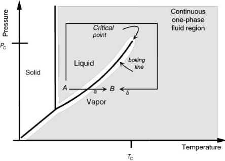
We usually think of a transition of a pure material from its liquid state to its gaseous state as requiring a discontinuous phase change, i.e. boiling. This is depicted by path a in Figure 7.1 in which we transform pure liquid water at ambient conditions, A, to its gaseous form at 150oC, B, by heating at constant, atmospheric pressure. Once again, this discontinuous change, our normal expectation, results from

Figure 7.1 Representation of the phase diagram for a pure fluid such as water. The shaded area is the continuum through which we can continuously vary the properties of the fluid. The high-pressure and high-temperature limits shown here are arbitrary. They depend only on the capabilities of the experimental apparatus and the stability of the apparatus and the fluid.

154	Multidimensional Chromatography

our experiences of living our entire lives at ambient pressure. However, in actuality, there is a continuum of fluid behavior linking the normal liquid and gas states, shown by the shaded area in the figure. In order to avoid discontinuities, we simply need to place the phase transitions off limits.

By traveling within the continuum and avoiding the boiling line, we can convert the ordinary liquid to its gaseous form without undergoing a phase change. One path accomplishing this is path b in the figure. Of course, an unlimited number of such paths is possible. The only requirement for continuous change is that we never cross the boiling line. Instead, we will go around the critical point, the point at which liquid and vapor states merge into a single fluid with shared properties.

Now, we should ask ourselves about the properties of water in this continuum of behavior mapped with temperature and pressure coordinates. First, let us look at temperature influence. The viscosity of the liquid water and its dielectric constant both drop when the temperature is raised (19). The balance between hydrogen bonding and other interactions changes. The diffusion rates increase with temperature. These dependencies on temperature provide us with an opportunity to tune the solvation properties of the liquid and change the relative solubilities of dissolved solutes without invoking a chemical composition change on the water.

If the property changes that occur when we raise the temperature are useful to us, and if we would like to continue moving continuously in the direction of these improvements, we are not limited by the normal boiling point. We simply need to apply enough pressure to prevent boiling, and then continue going on with our temperature exploration. Pressure does have a measurable effect on the solvent properties of liquids and on the relative retention of solutes in LC (20), but this effect is small in liquids at ordinary pressures and is usually ignored. However, the compressibility of the liquid and the effect of pressure both increase with increasing temperature.

Thus, there is not necessarily a boundary at the normal boiling point when we control the pressure. Why would we not want to take full advantage of the full range of properties of water, or of any other solvent, whenever advantages discovered away from ambient conditions improve our ability to separate solutes of interest?

Of course, LC is not often carried out with neat mobile-phase fluids. As we blend solvents we must pay attention to the phase behavior of the mixtures we produce. This adds complexity to the picture, but the same basic concepts still hold: we need to define the region in the phase diagram where we have continuous behavior and only one fluid state. For a two-component mixture, the complete phase diagram requires three dimensions, as shown in Figure 7.2. This figure represents a Type I mixture, meaning the two components are miscible as liquids. There are numerous other mixture types (21), many with miscibility gaps between the components, but for our purposes the Type I mixture is sufficient.

The shaded region is that part of the phase diagram where liquid and vapor phases coexist in equilibrium, somewhat in analogy to the boiling line for a pure fluid. The ordinary liquid state exists on the high-pressure, low-temperature side of the twophase region, and the ordinary gas state exists on the other side at low pressure and high temperature. As with our earlier example, we can transform any Type I mixture

Unified Chromatography

155

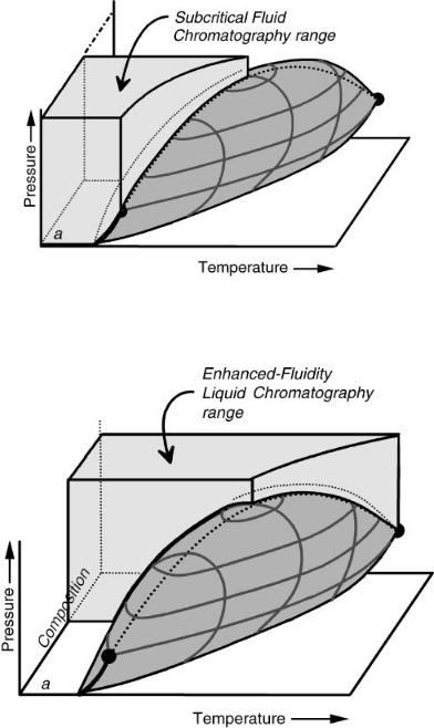
Figure 7.2 A three-dimensional phase diagram for a Type I binary mixture (here, CO2 and methanol). The shaded volume is the two-phase liquid-vapor region. This is shown truncated at 25 °C for illustration purposes. The volume surrounding the two-phase region is the continuum of fluid behavior.

from its liquid state to its gaseous state in a completely continuous manner by changing the pressure and temperature to simply go around the two-phase region of the figure. We can further continuously change the nature of the fluid by changing its composition. We are completely free to do so in a Type I mixture without realizing a discontinuity of any sort as long as we avoid the two-phase region (and, of course, the solid region, not shown, existing at lower temperatures). Now we have quite a large range of continuous behavior available to us, represented by the volume of the figure outside the forbidden two-phase region and limited only by the temperature and pressure capabilities of our system.

Many chromatographic techniques have been named and are practiced in various regions of the fluid continuum. These regions are identified in Figures 7.3 – 7.8. We have not specified the mobile-phase components, and not all of these techniques are necessarily practical with the same mobile-phase component choices. However, the general view is valid.

LC is a limiting technique that occurs when the column outlet pressure is near ambient and we choose well-behaved liquids as our mobile phases. Our only means of adjusting solute retention (after selecting the stationary phase and the

156	Multidimensional Chromatography

Figure 7.3 The positions occupied by LC and GC in a generic Type I phase diagram representing the mobile phase. Note that the GC mobile phase is shown as being composed of 100% component a, but this makes no difference chemically because there are no solute – mobile-phase interactions in GC. Reproduced by permission of the American Chemical Society.

mobile-phase components) is to vary the composition of the mobile phase, as indicated by the LC arrow in Figure 7.3. Although pressure is elevated at the column inlet, its only purpose is to generate mobile-phase flow. Pressure provides virtually no opportunity for adjusting retention or selectivity in conventional high-perfor- mance LC (HPLC). High-temperature LC is practiced simply by raising the column temperature. It provides some new benefits, of course, but is limited by the normal boiling point of the mobile phase unless significant pressure is applied at the column outlet.

When the pressure is controlled over a substantial range, we can more fully enter the subcritical fluid chromatography (SubFC) and enhanced-fluidity liquid chromatography (EFLC) (22, 23) regions shown in Figures 7.4 and 7.5, respectively. Both of these techniques are performed below the critical temperature locus of the mobile phase. Both of them frequently take advantage of very volatile mobile-phase components in order to maximize diffusion rates and speed of analysis. The only difference between these techniques is which fluid is denoted as being the main fluid. In SubFC, the more-volatile mobile-phase component is considered to be the main component, while the less-volatile component is considered to be a modifier used to change solvation characteristics. In EFLC, the less-volatile component is considered to be the main component, and the more-volatile component is considered to be a viscosity (and diffusion) enhancer. Clearly, there is no chemically meaningful boundary between SubFC and EFLC.

Unified Chromatography

157

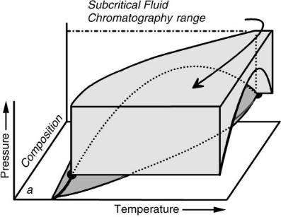
Figure 7.4 The Subcritical Fluid Chromatography range. This occupies the volume in the phase diagram below the locus of critical temperatures, above and below the locus of critical pressures, and is composed mostly of the more volatile mobile-phase component. Reproduced by permission of the American Chemical Society.

Figure 7.5 The Enhanced Fluidity Liquid Chromatography range. This occupies the volume in the phase diagram below the locus of critical temperatures, above and below the locus of critical pressures, and is composed mostly of the less volatile mobile-phase component. Reproduced by permission of the American Chemical Society.

158	Multidimensional Chromatography

Figure 7.6 The Supercritical Fluid Chromatography range, above both the critical temperature and pressure at all compositions. (Reprinted with permission from reference 17. Copyright 1997 American Chemical Society.) Reproduced by permission of the American Chemical Society.

SFC (see Figure 7.6) occurs when both the critical temperature and critical pressure of the mobile phase are exceeded. (The locus of critical points is indicated in Figure 7.2 by the dashed line over the top of the two-phase region. It is also visible or partly visible in Figures 7.3 – 7.8). Compressibility, pressure tunability, and diffusion rates are higher in SFC than in SubFC and EFLC, and are much higher than in LC.

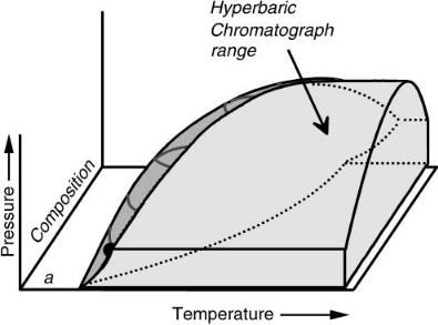
We have denoted the next region as hyperbaric chromatography (see Figure 7.7) where temperatures are above the two-phase boundary and pressure is below critical. In this region, the compressibility of the mobile phase is higher than in the previously described regions. However, the solvent is not as strong, in general, because the decrease in pressure and the expansion of the compressible mobile phase increase intermolecular distances and reduce solute – mobile-phase interactions. Solvating gas chromatography (SGC) is a limiting case of hyperbaric chromatography in which the column outlet is allowed to default to one atmosphere (24).

Mobile phases with some solvating potential, such as CO2 or ammonia, are necessary in SGC. Even though this technique is performed with ambient outlet pressure, solutes can be separated at lower temperatures than in GC because the average pressure on the column is high enough that solvation occurs. Obviously, solute retention is not constant in the column, and the local values of retention factors increase for all solutes as they near the column outlet.

Unified Chromatography

159

Figure 7.7 The Hyperbaric Chromatography region, at temperatures above the 2-phase region and pressures below the locus of critical pressures. Reproduced by permission of the American Chemical Society.

As we continue lowering the pressure, GC is the final limiting case when the mobile phase has zero solvent strength over the entire column length and where temperature is the only effective control parameter. Gas chromatography is shown in Figure 7.3.

Our view of unified chromatography simply involves realizing that the technique names and the boundaries defining them are arbitrary definitions lacking any real meaning with respect to fluid behavior, except perhaps when ambient conditions are invoked by default. In order to perceive unified chromatography, we simply eliminate the arbitrary boundaries separating the adjacent techniques and merge or unify all these techniques into one, as shown in Figure 7.8. We are also now completely free to select the conditions that produce the best separation for a particular problem from anywhere within this continuum of behavior without regard to naming conventions or arbitrary restrictions. We will probably want to avoid the two-phase region under most circumstances, and are limited in temperature and pressure only by the capabilities and stability of the instrument, stationary phase and solutes.

7.3INSTRUMENTATION

The basic instrument required for packed-column unified chromatography is shown schematically in Figure 7.9. This is essentially a two-pump HPLC instrument utilizing high-pressure mixing with just a few new components. At least one pump must